Competing Failure Modes Analysis
Often, a group of products will fail due to more than one failure mode. One can take the view that the products could have failed due to any one of the possible failure modes, but since an item cannot fail more than one time, there can only be one failure mode for each failed product. In this view, the failure modes compete as to which causes the failure for each particular item. This can be viewed as a series system reliability model, with each failure mode composing a block of the series system. Competing failure modes (CFM) analysis segregates the analyses of failure modes and then combines the results to provide an overall model for the product in question.
CFM Analysis Approach
In order to begin analyzing data sets with more than one competing failure mode, one must perform a separate analysis for each failure mode. During each of these analyses, the failure times for all other failure modes not being analyzed are considered to be suspensions. This is because the units under test would have failed at some time in the future due to the failure mode being analyzed, had the unrelated (not analyzed) mode not occurred. Thus, in this case, the information available is that the mode under consideration did not occur and the unit under consideration accumulated test time without a failure due to the mode under consideration (or a suspension due to that mode).
Once the analysis for each separate failure mode has been completed (using the same principles as before), the resulting reliability equation for all modes is the product of the reliability equation for each mode, or:
where is the total number of failure modes considered. This is the product rule for the reliability of series systems with statistically independent components, which states that the reliability for a series system is equal to the product of the reliability values of the components comprising the system. Do note that the above equation is the reliability function based on any assumed life distribution. In Weibull++ this life distribution can be either the 2-parameter Weibull, lognormal, normal or the 1-parameter exponential.
CFM Example
The following example demonstrates how you can use the reliability equation to determine the overall reliability of a component. (This example has been abstracted from Example 15.6 from the Meeker and Escobar textbook Statistical Methods for Reliability Data [27].)
An electronic component has two competing failure modes. One failure mode is due to random voltage spikes, which cause failure by overloading the system. The other failure mode is due to wearout failures, which usually happen only after the system has run for many cycles. The objective is to determine the overall reliability for the component at 100,000 cycles.
30 units are tested, and the failure times are recorded in the following table. The failures that are due to the random voltage spikes are denoted by a V. The failures that are due to wearout failures are denoted by a W.
| Number in State | Failure Time* | Failure Mode | Number in State | Failure Time* | Failure Mode |
|---|---|---|---|---|---|
| 1 | 2 | V | 1 | 147 | W |
| 1 | 10 | V | 1 | 173 | V |
| 1 | 13 | V | 1 | 181 | W |
| 2 | 23 | V | 1 | 212 | W |
| 1 | 28 | V | 1 | 245 | W |
| 1 | 30 | V | 1 | 247 | V |
| 1 | 65 | V | 1 | 261 | V |
| 1 | 80 | V | 1 | 266 | W |
| 1 | 88 | V | 1 | 275 | W |
| 1 | 106 | V | 1 | 293 | W |
| 1 | 143 | V | 1 | 300 | suspended |
*Failure times given are in thousands of cycles.
Solution
To obtain the overall reliability of the component, we will first need to analyze the data set due to each failure mode. For example, to obtain the reliability of the component due to voltage spikes, we must consider all of the failures for the wear-out mode to be suspensions. We do the same for analyzing the wear-out failure mode, counting only the wear-out data as failures and assuming that the voltage spike failures are suspensions. Once we have obtained the reliability of the component due to each mode, we can use the system Reliability Equation to determine the overall component reliability.
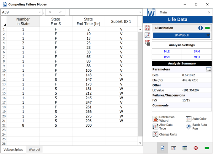
The following analysis shows the data set for the voltage spikes. Using the Weibull distribution and the MLE analysis method (recommended due to the number of suspensions in the data), the parameters are
and
. The reliability for this failure mode at
is
.
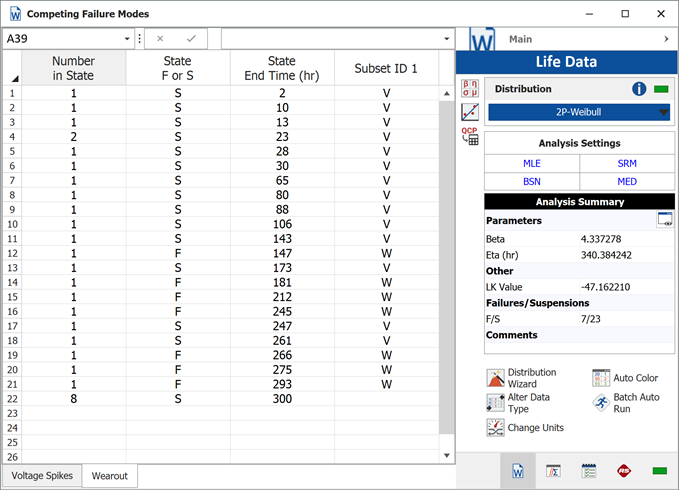
The following analysis shows the data set for the wearout failure mode. Using the same analysis settings (i.e., Weibull distribution and MLE analysis method), the parameters are
and
. The reliability for this failure mode at
is
.
Using the Reliability Equation to obtain the overall component reliability at 100,000 cycles, we get:
Or the reliability of the unit (or system) under both modes is
.
You can also perform this analysis using Weibull++'s built-in CFM analysis options, which allow you to generate a probability plot that contains the combined mode line as well as the individual mode lines.
Confidence Bounds for CFM Analysis
The method available in Weibull++ for estimating the different types of confidence bounds, for competing failure modes analysis, is the Fisher matrix method, and is presented in this section.
Variance/Covariance Matrix
The variances and covariances of the parameters are estimated from the inverse local Fisher matrix, as follows:
where is the log-likelihood function of the failure distribution, described in
Parameter Estimation.
Bounds on Reliability
The competing failure modes reliability function is given by:
where:
is the reliability of the
mode.
is the number of failure modes.
The upper and lower bounds on reliability are estimated using the logit transformation:
where is calculated using the reliability equation for competing failure modes.
is defined by:
(If is the confidence level, then
for the two-sided bounds, and
for the one-sided bounds.)
The variance of is estimated by:
Thus:
where is an element of the model parameter vector.
Therefore, the value of is dependent on the underlying distribution.
For the Weibull distribution:
where:
and is given in
The Weibull Distribution.
For the exponential distribution:
where is given in
The Exponential Distribution.
For the normal distribution:
where is given in
The Normal Distribution.
For the lognormal distribution:
where is given in
The Lognormal Distribution.
Bounds on Time
The bounds on time are estimate by solving the reliability equation with respect to time. From the reliabilty equation for competing faiure modes, we have that:
where:
-
-
is inverse function for the reliabilty equation for competing faiure modes.
- for the Weibull distribution
is
, and
is
- for the exponential distribution
is
, and
=0
- for the normal distribution
is
, and
is
, and
- for the lognormal distribution
is
, and
is
-
Set:
The bounds on are estimated from:
and:
Then the upper and lower bounds on time are found by using the equations:
and:
is calculated using the inverse standard normal distribution and
is computed as:
Complex Failure Modes Analysis
In addition to being viewed as a series system, the relationship between the different competing failures modes can be more complex. After performing separate analysis for each failure mode, a diagram that describes how each failure mode can result in a product failure can be used to perform analysis for the item in question. Such diagrams are usually referred to as Reliability Block Diagrams (RBD) (for more on RBDs see ReliaSoft's System Analysis Reference and ReliaSoft's BlockSim software).
A reliability block diagram is made of blocks that represent the failure modes and arrows and connects the blocks in different configurations. Note that the blocks can also be used to represent different components or subsystems that make up the product. Weibull++ provides the capability to use a diagram to model, series, parallel, k-out-of-n configurations in addition to any complex combinations of these configurations.
In this analysis, the failure modes are assumed to be statistically independent. (Note: In the context of this reference, statistically independent implies that failure information for one failure mode provides no information about, i.e. does not affect, other failure mode). Analysis of dependent modes is more complex. Advanced RBD software such as ReliaSoft's BlockSim can handle and analyze such dependencies, as well as provide more advanced constructs and analyses.
Failure Modes Configurations
Series Configuration
The basic competing failure modes configuration, which has already been discussed, is a series configuration. In a series configuration, the occurrence of any failure mode results in failure for the product.
The equation that describes series configuration is:
where is the total number of failure modes considered.
Parallel
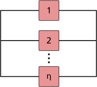
In a simple parallel configuration, at least one of the failure modes must not occur for the product to continue operation.
The equation that describes the parallel configuration is:
where is the total number of failure modes considered.
Combination of Series and Parallel
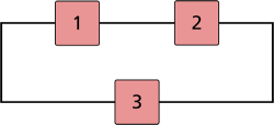
While many smaller products can be accurately represented by either a simple series or parallel configuration, there may be larger products that involve both series and parallel configurations in the overall model of the product. Such products can be analyzed by calculating the reliabilities for the individual series and parallel sections and then combining them in the appropriate manner.
k-out-of-n Parallel Configuration=
The k-out-of-n configuration is a special case of parallel redundancy. This type of configuration requires that at least
failure modes do not happen out of the total
parallel failure modes for the product to succeed.
The simplest case of a k-out-of-n configuration is when the failure modes are independent and identical and have the same failure distribution and uncertainties about the parameters (in other words they are derived from the same test data). In this case, the reliability of the product with such a configuration can be evaluated using the binomial distribution, or:
In the case where the k-out-of-n failure modes are not identical, other approaches for calculating the reliability must be used (e.g. the event space method). Discussion of these is beyond the scope of this reference. Interested readers can consult the System Analysis Reference book.
Complex Systems
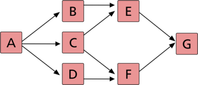
In many cases, it is not easy to recognize which components are in series and which are in parallel in a complex system.
The previous configuration cannot be broken down into a group of series and parallel configurations. This is primarily due to the fact that failure mode C has two paths leading away from it, whereas B and D have only one. Several methods exist for obtaining the reliability of a complex configuration including the decomposition method, the event space method and the path-tracing method. Discussion of these is beyond the scope of this reference. Interested readers can consult the System Analysis Reference book.
Complex Failure Modes Example
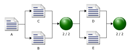
Assume that a product has five independent failure modes: A, B, C, D and E. Furthermore, assume that failure of the product will occur if mode A occurs, modes B and C occur simultaneously or if modes D and E occur simultaneously. The objective is to estimate the reliability of the product at 100 hours, with 90% two-sided confidence bounds.
The product is tested to failure, and the failure times due to each mode are recorded in the following table.
| TTF for A | TTF for B | TTF for C | TTF for D | TTF for E |
|---|---|---|---|---|
| 276 | 23 | 499 | 467 | 67 |
| 320 | 36 | 545 | 540 | 72 |
| 323 | 57 | 661 | 716 | 81 |
| 558 | 89 | 738 | 737 | 108 |
| 674 | 99 | 987 | 761 | 110 |
| 829 | 154 | 1165 | 1093 | 127 |
| 878 | 200 | 1337 | 1283 | 148 |
Solution
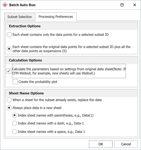
The reliability block diagram (RBD) approach can be used to analyze the reliability of the product. But before creating a diagram, the data sets of the failure modes need to be segregated so that each mode can be represented by a single block in the diagram. Recall that when you analyze a particular mode, the failure times for all other competing modes are considered to be suspensions. This captures the fact that those units operated for a period of time without experiencing the failure mode of interest before they were removed from observation when they failed due to another mode. We can easily perform this step via Weibull++'s Batch Auto Run utility. To do this, enter the data from the table into a single data sheet. Choose the 2P-Weibull distribution and the MLE analysis method, and then click the Batch Auto Run icon on the control panel. When prompted to select the subset IDs, select them all. Click the Processing Preferences tab. In the Extraction Options area, select the second option, as shown next.
This will extract the data sets that are required for the analysis. Select the check box in the Calculation Options area and click OK. The data sets are extracted into separate data sheets in the folio and automatically calculated.
Next, create a diagram by choosing Home > Insert > Diagram. Add blocks by right-clicking the diagram and choosing Add Block on the shortcut menu. When prompted to select the data sheet of the failure mode that the block will represent, select the data sheet for mode A. Use the same approach to add the blocks that will represent failure modes B, C , D and E. Add a connector by right-clicking the diagram sheet and choosing Connect Blocks, and then connect the blocks in an appropriate configuration to describe the relationships between the failure modes. To insert a node, which acts as a switch that the diagram paths move through, right-click the diagram and choose Add Node. Specify the number of required paths in the node by double-clicking the node and entering the appropriate number (use 2 in both nodes).
The following figure shows the completed diagram.
Click Analyze to analyze the diagram, and then use the Quick Calculation Pad (QCP) to estimate the reliability. The estimated R(100 hours) and the 90% two-sided confidence bounds are:


