Basics of System Reliability Analysis

Overview

In life data analysis and accelerated life testing data analysis, as well as other testing activities, one of the primary objectives is to obtain a life distribution that describes the times-to-failure of a component, subassembly, assembly or system. This analysis is based on the time of successful operation or time-to-failure data of the item (component), either under use conditions or from accelerated life tests.

For any life data analysis, the analyst chooses a point at which no more detailed information about the object of analysis is known or needs to be considered. At that point, the analyst treats the object of analysis as a "black box." The selection of this level (e.g., component, subassembly, assembly or system) determines the detail of the subsequent analysis.

In system reliability analysis, one constructs a "System" model from these component models. In other words in system reliability analysis we are concerned with the construction of a model (life distribution) that represents the times-to-failure of the entire system based on the life distributions of the components, subassemblies and/or assemblies ("black boxes") from which it is composed, as illustrated in the figure below.

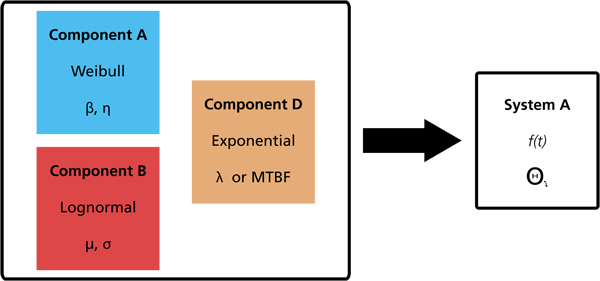
To accomplish this, the relationships between components are considered and decisions about the choice of components can be made to improve or optimize the overall system reliability, maintainability and/or availability. There are many specific reasons for looking at component data to estimate the overall system reliability. One of the most important is that in many situations it is easier and less expensive to test components/subsystems rather than entire systems. Many other benefits of the system reliability analysis approach also exist and will be presented throughout this reference.

Systems

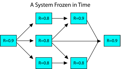
A system is a collection of components, subsystems and/or assemblies arranged to a specific design in order to achieve desired functions with acceptable performance and reliability. The types of components, their quantities, their qualities and the manner in which they are arranged within the system have a direct effect on the system's reliability. The relationship between a system and its components is often misunderstood or oversimplified. For example, the following statement is not valid: All of the components in a system have a 90% reliability at a given time, thus the reliability of the system is 90% for that time. Unfortunately, poor understanding of the relationship between a system and its constituent components can result in statements like this being accepted as factual, when in reality they are false.

Reliability Block Diagrams (RBDs)

Block diagrams are widely used in engineering and science and exist in many different forms. They can also be used to describe the interrelation between the components and to define the system. When used in this fashion, the block diagram is then referred to as a reliability block diagram (RBD).

A reliability block diagram is a graphical representation of the components of the system and how they are reliability-wise related (connected). It should be noted that this may differ from how the components are physically connected. An RBD of a simplified computer system with a redundant fan configuration is shown below.

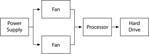
RBDs are constructed out of blocks. The blocks are connected with direction lines that represent the reliability relationship between the blocks.

A block is usually represented in the diagram by a rectangle. In a reliability block diagram, such blocks represent the component, subsystem or assembly at its chosen black box level. The following figure shows two blocks, one representing a resistor and one representing a computer.

It is possible for each block in a particular RBD to be represented by its own reliability block diagram, depending on the level of detail in question. For example, in an RBD of a car, the top level blocks could represent the major systems of the car, as illustrated in the figure below. Each of these systems could have their own RBDs in which the blocks represent the subsystems of that particular system. This could continue down through many levels of detail, all the way down to the level of the most basic components (e.g., fasteners), if so desired.

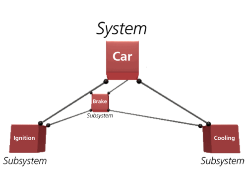
The level of granularity or detail that one chooses should be based on both the availability of data and on the lowest actionable item concept. To illustrate this concept, consider the aforementioned computer system shown earlier. When the computer manufacturer finds out that the hard drive is not as reliable as it should be and decides not to try to improve the reliability of the current hard drive but rather to get a new hard drive supplier, then the lowest actionable item is the hard drive. The hard drive supplier will then have actionable items inside the hard drive, and so forth.

Block Failure Models

Having segmented a product or process into parts, the first step in evaluating the reliability of a system is to obtain life/event data concerning each component/subsystem (i.e., each block). This information will allow the reliability engineer to characterize the life distribution of each component. Data can be obtained from different sources, including:

• In-house reliability tests
• Accelerated life tests
• Field data
• Warranty data
• Engineering knowledge
• Similarity to prior designs
• Other reference sources

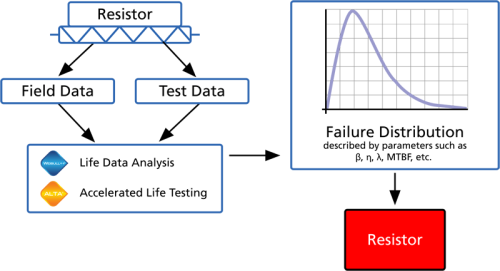
Additionally, component life data may also be provided by the manufacturer or supplier of the component/subsystem. Once the data set has been obtained, the life distribution of a component/subsystem can be estimated using ReliaSoft's Weibull++ or ALTA software. For example, consider a resistor that is part of a larger system to be analyzed. Failure data for this resistor can be obtained by performing in-house reliability tests and by observing the behavior of that type of resistor in the field. As shown below, a life distribution is then fitted to the data and the parameters are obtained. The parameters of that distribution represent the life distribution of that resistor block in the overall system RBD.

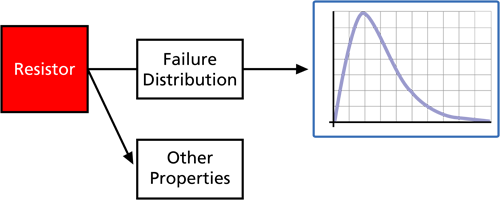
In the same manner, other types of information can also be obtained that can be used to define other block properties, such as the time-to-repair distribution (by analyzing the times-to-repair of each block instead of the times-to-failure), other maintenance requirements, throughput properties, etc. These block properties can then be used to perform a variety of analyses on the overall system to predict and/or optimize the system's reliability, maintainability, availability, spare parts utilization, throughput, etc.

Available Distributions

Because the failure properties of a component are best described by statistical distributions, the most commonly used life distributions are available in BlockSim. (For more information about these distributions, see Life Distributions.) The available distributions are:

• 1 and 2 parameter exponential distributions
• 1, 2 and 3 parameter Weibull distributions
• Mixed Weibull distribution (with 2, 3 or 4 subpopulations)
• Normal distribution
• Lognormal distribution
• Generalized-Gamma (i.e., G-Gamma) distribution
• Gamma distribution
• Logistic distribution
• Loglogistic distribution
• Gumbel distribution

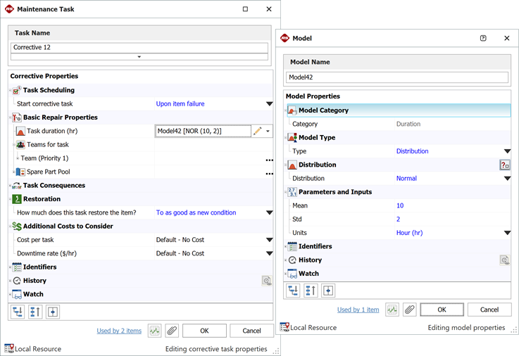
The same distributions are also available as repair distributions and in other probabilistic property windows that we will discuss later. The first figure below illustrates the Block Properties window with the Weibull distribution assigned as the failure distribution while the second figure illustrates the Block Properties window with the normal distribution assigned as the repair distribution.

System Reliability Function

After defining the properties of each block in a system, the blocks can then be connected in a reliability-wise manner to create a reliability block diagram for the system. The RBD provides a visual representation of the way the blocks are reliability-wise arranged. This means that a diagram will be created that represents the functioning state (i.e., success or failure) of the system in terms of the functioning states of its components. In other words, this diagram demonstrates the effect of the success or failure of a component on the success or failure of the system. For example, if all components in a system must succeed in order for the system to succeed, the components will be arranged reliability-wise in series. If one of two components must succeed in order for the system to succeed, those two components will be arranged reliability-wise in parallel. RBDs and Analytical System Reliability discusses RBDs and diagramming methods.

The reliability-wise arrangement of components is directly related to the derived mathematical description of the system. The mathematical description of the system is the key to the determination of the reliability of the system. In fact, the system's reliability function is that mathematical description (obtained using probabilistic methods) and it defines the system reliability in terms of the component reliabilities. The result is an analytical expression that describes the reliability of the system as a function of time based on the reliability functions of its components. Statistical Background, RBDs and Analytical System Reliability and Time-Dependent System Reliability (Analytical) discuss this further. These chapters also offer derivations of needed equations and present examples.

Non-Repairable and Repairable Systems

Systems can be generally classified into non-repairable and repairable systems. Non-repairable systems are those that do not get repaired when they fail. Specifically, the components of the system are not repaired or replaced when they fail. Most household products, for example, are non-repairable. This does not necessarily mean that they cannot be repaired, but rather that it does not make economic sense to do so. For example, repairing a four-year-old microwave oven is economically unreasonable, since the repair would cost approximately as much as purchasing a new unit.

On the other hand, repairable systems are those that get repaired when they fail. This is done by repairing or replacing the failed components in the system. An automobile is an example of a repairable system. If the automobile is rendered inoperative when a component or subsystem fails, that component is typically repaired or replaced rather than purchasing a new automobile. In repairable systems, two types of distributions are considered: failure distributions and repair distributions. A failure distribution describes the time it takes for a component to fail. A repair distribution describes the time it takes to repair a component (time-to-repair instead of time-to-failure). In the case of repairable systems, the failure distribution itself is not a sufficient measure of system performance, since it does not account for the repair distribution. A new performance criterion called availability can be calculated, which accounts for both the failure and repair distributions.

Repairable systems and availability will be discussed in Introduction to Repairable Systems and Repairable Systems Analysis Through Simulation.

BlockSim's Computation Modes

As shown in the figure below, BlockSim includes two independent computation modes: analytical and simulation. The analytical mode uses the exact reliability solutions for the system, employing the system's reliability function or cumulative density function (cdf). BlockSim can resolve even the most complex systems analytically and this method should be used when one is performing reliability analysis. In the context of BlockSim and this reference, we use the term reliability analysis to refer to all analyses that do not include repairs or restorations of the component. In contrast to the analytical mode, the simulation mode takes into account repair and restoration actions, including behaviors of crews, spare part pools, throughput, etc. Both of these methods will be explored in the chapters that follow.

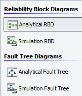
When considering only the failure characteristics of the components, the analytical approach should be used. However, when both the failure and maintenance characteristics need to be considered, the simulation method must be used to take into account the additional events.

Analytical Calculations

In the analytical (or algebraic analysis) approach, the system's pdf is obtained analytically from each component's failure distribution using probability theory. In other words, the analytical approach involves the determination of a mathematical expression that describes the reliability of the system in terms the reliabilities of its components. Remember also that .

The advantages of the analytical approach are:

• The mathematical expression for the system's cdf is obtained.
• Conditional reliability, warranty time and other calculations can be performed.
• Ancillary analyses can be performed, such as optimized reliability allocation, reliability importance computation of components, etc.

The disadvantage of the analytical approach is:

• Analyses that involve repairable systems with multiple additional events and/or other maintainability information are very difficult (if not impossible) to solve analytically. In these cases, analysis through simulation becomes necessary.
  

Two types of analytical calculations can be performed using RBDs (and BlockSim): static reliability calculations and time-dependent reliability calculations. Systems can contain static blocks, time-dependent blocks or a mixture of the two. Analytical computations are discussed in RBDs and Analytical System Reliability and Time-Dependent System Reliability (Analytical).

Static

Static analytical calculations are performed on RBDs that contain static blocks. A static block can be interpreted either as a block with a reliability value that is known only at a given time (but the block's entire distribution is unknown) or as a block with a probability of success that is constant with time. Static calculations can be performed both in the analytical mode and the simulation mode. The following figure illustrates a static RBD.

Time-Dependent

Time-dependent analysis looks at reliability as a function of time. That is, a known failure distribution is assigned to each component. The time scale in BlockSim can assume any quantifiable time measure, such as years, months, hours, minutes or seconds, and also units that are not directly related to time, such as cycles or miles of use. 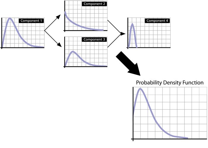In many of the discussions and examples that follow, and to maintain generality, time units may be omitted or a general time unit ( ) may be utilized. It is very important to remember that even though any time unit may be used, the time units used throughout an analysis must be consistent in order to avoid incorrect results. The primary objective in system reliability analysis is to obtain a failure distribution of the entire system based on the failure distributions of its components, as illustrated below.

Simulation Calculations

If one includes information on the repair and maintenance characteristics of the components and resources available in the system, other information can also be analyzed/obtained, such as system availability, throughput, spare parts usage, life costs, etc. This can be accomplished through discrete event simulation.

In simulation, random failure times from each component's failure distribution are generated. These failure times are then combined in accordance with the way the components are reliability-wise arranged within the system. The overall results are analyzed in order to determine the behavior of the entire system.

The advantages of the simulation approach are:

• It can be used for highly complex scenarios involving a multitude of probabilistic events, such as corrective maintenance, preventive maintenance, inspections, imperfect repairs, crew response times, spare part availability, etc. When events such as these are considered, analytical solutions become impossible when dealing with real systems of sufficient complexity.
• The discrete event simulation also has the capabilities for:
  • Examining resource usage, efficiency and costs.
  • Optimizing procedures and resource allocation.
  • Analyzing relationships between systems and components.
  • Maximizing throughput.
  • Minimizing work downtimes.

The disadvantages of the simulation approach are:

• It can be time-consuming.
• The results are dependent on the number of simulations.
• There is a lack of repeatability in the results due to the random nature of data generation.

Simulation is discussed in the Repairable Systems Analysis Through Simulation and Throughput Analysis chapters.