Statistical Background
This chapter presents a brief review of statistical principles and terminology. The objective of this chapter is to introduce concepts from probability theory and statistics that will be used in later chapters. As such, this chapter is not intended to cover this subject completely, but rather to provide an overview of applicable concepts as a foundation that you can refer to when more complex concepts are introduced.
If you are familiar with basic probability theory and life data analysis, you may wish to skip this chapter. If you would like additional information, we encourage you to review other references on the subject.
A Brief Introduction to Probability Theory
Basic Definitions
Before considering the methodology for estimating system reliability, some basic concepts from probability theory should be reviewed.
The terms that follow are important in creating and analyzing reliability block diagrams.
- Experiment
: An experiment is any well-defined action that may result in a number of outcomes. For example, the rolling of dice can be considered an experiment.
- Outcome
: An outcome is defined as any possible result of an experiment.
- Sample space
: The sample space is defined as the set of all possible outcomes of an experiment.
- Event: An event is a collection of outcomes.
- Union of two events
and
: The union of two events
and
is the set of outcomes that belong to
or
or both.
- Intersection of two events
and
: The intersection of two events
and
is the set of outcomes that belong to both
and
.
- Complement of event A (
): A complement of an event
contains all outcomes of the sample space,
, that do not belong to
.
- Null event (
): A null event is an empty set that has no outcomes.
- Probability: Probability is a numerical measure of the likelihood of an event relative to a set of alternative events. For example, there is a 50% probability of observing heads relative to observing tails when flipping a coin (assuming a fair or unbiased coin).
Example
Consider an experiment that consists of the rolling of a six-sided die. The numbers on each side of the die are the possible outcomes. Accordingly, the sample space is
.
Let be the event of rolling a 3, 4 or 6,
, and let
be the event of rolling a 2, 3 or 5,
.
- The union of
and
is:
.
- The intersection of
and
is:
.
- The complement of
is:
.
Probability Properties, Theorems and Axioms
The probability of an event is expressed as
and has the following properties:
In other words, when an event is certain to occur, it has a probability equal to 1; when it is impossible for the event to occur, it has a probability equal to 0.
It can also be shown that the probability of the union of two events
and
is:
Similarly, the probability of the union of three events,
,
and
is given by:
Mutually Exclusive Events
Two events and
are said to be mutually exclusive if it is impossible for them to occur simultaneously (
=
). In such cases, the expression for the union of these two events reduces to the following, since the probability of the intersection of these events is defined as zero.
Conditional Probability
The conditional probability of two events
and
is defined as the probability of one of the events occurring, knowing that the other event has already occurred. The expression below denotes the probability of
occurring given that
has already occurred.
Note that knowing that event has occurred reduces the sample space.
Independent Events
If knowing gives no information about
, then the events are said to be
independent and the conditional probability expression reduces to:
From the definition of conditional probability,
can be written as:
Since events and
are independent, the expression reduces to:
If a group of events
are independent, then:
As an illustration, consider the outcome of a six-sided die roll. The probability of rolling a 3 is one out of six or:
All subsequent rolls of the die are independent events, since knowing the outcome of the first die roll gives no information as to the outcome of subsequent die rolls (unless the die is loaded). Thus the probability of rolling a 3 on the second die roll is again:
However, if one were to ask the probability of rolling a double 3 with two dice, the result would be:
Example 1
Consider a system where two hinged members are holding a load in place, as shown next.
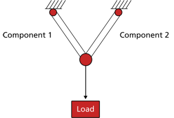
The system fails if either member fails and the load is moved from its position.
- Let
event of failure of Component 1 and let
the event of not failure of Component 1.
- Let
event of failure of Component 2 and let
the event of not failure of Component 2.
Failure occurs if Component 1 or Component 2 or both fail. The system probability of failure (or unreliability) is:
Assuming independence (or that the failure of either component is not influenced by the success or failure of the other component), the system probability of failure becomes the sum of the probabilities of
and
occurring minus the product of the probabilities:
Another approach is to calculate the probability of the system not failing (i.e., the reliability of the system):
Then the probability of system failure is simply 1 (or 100%) minus the reliability:
Example 2
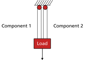
Consider a system with a load being held in place by two rigid members, as shown next.
- Let
event of failure of Component 1.
- Let
event of failure of Component 2.
- The system fails if Component 1 fails and Component 2 fails. In other words, both components must fail for the system to fail.
The system probability of failure is defined as the intersection of events
and
:
Case 1
Assuming independence (i.e., either one of the members is sufficiently strong to hold the load in place), the probability of system failure becomes the product of the probabilities of
and
failing:
The reliability of the system now becomes:
Case 2
If independence is not assumed (e.g., when one component fails the other one is then more likely to fail), then the simplification given in
is no longer applicable. In this case,
must be used. We will examine this dependency in later sections under the subject of load sharing.
A Brief Introduction to Continuous Life Distributions
Random Variables

In general, most problems in reliability engineering deal with quantitative measures, such as the time-to-failure of a component, or qualitative measures, such as whether a component is defective or non-defective. We can then use a random variable
to denote these possible measures.
In the case of times-to-failure, our random variable
is the time-to-failure of the component and can take on an infinite number of possible values in a range from 0 to infinity (since we do not know the exact time
a priori). Our component can be found failed at any time after time 0 (e.g., at 12 hours or at 100 hours and so forth), thus
can take on any value in this range. In this case, our random variable
is said to be a
continuous random variable. In this reference, we will deal almost exclusively with continuous random variables.
In judging a component to be defective or non-defective, only two outcomes are possible. That is,
is a random variable that can take on one of only two values (let's say defective = 0 and non-defective = 1). In this case, the variable is said to be a discrete random variable.
The Probability Density Function and the Cumulative Distribution Function
The probability density function (pdf) and cumulative distribution function (cdf) are two of the most important statistical functions in reliability and are very closely related. When these functions are known, almost any other reliability measure of interest can be derived or obtained. We will now take a closer look at these functions and how they relate to other reliability measures, such as the reliability function and failure rate.
From probability and statistics, given a continuous random variable
we denote:
-
- The probability density function, pdf, as
.
- The probability density function, pdf, as
-
- The cumulative distribution function, cdf, as
.
- The cumulative distribution function, cdf, as
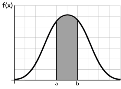
The pdf and cdf give a complete description of the probability distribution of a random variable. The following figure illustrates a pdf.
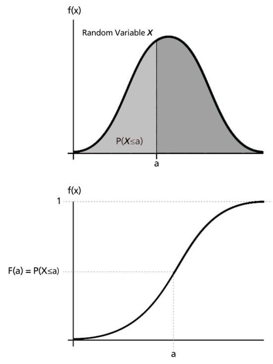
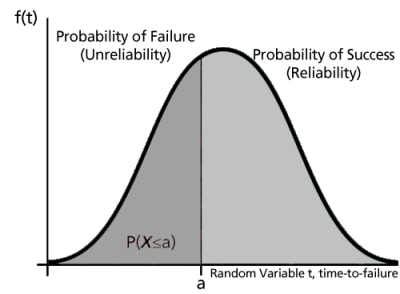
The next figures illustrate the pdf - cdf relationship.
If is a continuous random variable, then the
pdf of
is a function,
, such that for any two numbers,
and
with
:
That is, the probability that takes on a value in the interval
is the area under the density function from
to
as shown above. The
pdf represents the relative frequency of failure times as a function of time.
The cdf is a function, , of a random variable
, and is defined for a number
by:
That is, for a number ,
is the probability that the observed value of
will be at most
. The
cdf represents the cumulative values of the pdf. That is, the value of a point on the curve of the
cdf represents the area under the curve to the left of that point on the
pdf. In reliability, the cdf is used to measure the probability that the item in question will fail before the associated time value,
, and is also called
unreliability.
Note that depending on the density function, denoted by
, the limits will vary based on the region over which the distribution is defined. For example, for the life distributions considered in this reference, with the exception of the normal distribution, this range would be
Mathematical Relationship: pdf and cdf
The mathematical relationship between the pdf and cdf is given by:
where is a dummy integration variable.
Conversely:
The cdf is the area under the probability density function up to a value of
. The total area under the
pdf is always equal to 1, or mathematically:
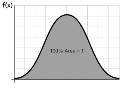
The well-known normal (or Gaussian) distribution is an example of a probability density function. The pdf for this distribution is given by:
where is the mean and
is the standard deviation. The normal distribution has two parameters,
and
.
Another is the lognormal distribution, whose pdf is given by:
where is the mean of the natural logarithms of the times-to-failure and
is the standard deviation of the natural logarithms of the times-to-failure. Again, this is a 2-parameter distribution.
Reliability Function
The reliability function can be derived using the previous definition of the cumulative distribution function,
. From our definition of the
cdf, the probability of an event occurring by time
is given by:
Or, one could equate this event to the probability of a unit failing by time
.
Since this function defines the probability of failure by a certain time, we could consider this the unreliability function. Subtracting this probability from 1 will give us the reliability function, one of the most important functions in life data analysis. The reliability function gives the probability of success of a unit undertaking a mission of a given time duration. The following figure illustrates this.
To show this mathematically, we first define the unreliability function,
, which is the probability of failure, or the probability that our time-to-failure is in the region of 0 and
. This is the same as the
cdf. So from
:
Reliability and unreliability are the only two events being considered and they are mutually exclusive; hence, the sum of these probabilities is equal to unity.
Then:
Conversely:
Conditional Reliability Function
Conditional reliability is the probability of successfully completing another mission following the successful completion of a previous mission. The time of the previous mission and the time for the mission to be undertaken must be taken into account for conditional reliability calculations. The conditional reliability function is given by:
Failure Rate Function
The failure rate function enables the determination of the number of failures occurring per unit time. Omitting the derivation, the failure rate is mathematically given as:
This gives the instantaneous failure rate, also known as the hazard function. It is useful in characterizing the failure behavior of a component, determining maintenance crew allocation, planning for spares provisioning, etc. Failure rate is denoted as failures per unit time.
Mean Life (MTTF)
The mean life function, which provides a measure of the average time of operation to failure, is given by:
This is the expected or average time-to-failure and is denoted as the MTTF (Mean Time To Failure).
The MTTF, even though an index of reliability performance, does not give any information on the failure distribution of the component in question when dealing with most lifetime distributions. Because vastly different distributions can have identical means, it is unwise to use the MTTF as the sole measure of the reliability of a component.
Median Life
Median life,
,
is the value of the random variable that has exactly one-half of the area under the
pdf to its left and one-half to its right.
It represents the centroid of the distribution.
The median is obtained by solving the following equation for
. (For individual data, the median is the midpoint value.)
Modal Life (or Mode)
The modal life (or mode), , is the value of
that satisfies:
For a continuous distribution, the mode is that value of
that corresponds to the maximum probability density (the value at which the
pdf has its maximum value, or the peak of the curve).
Lifetime Distributions
A statistical distribution is fully described by its pdf. In the previous sections, we used the definition of the
pdf to show how all other functions most commonly used in reliability engineering and life data analysis can be derived. The reliability function, failure rate function, mean time function, and median life function can be determined directly from the
pdf definition, or . Different distributions exist, such as the normal (Gaussian), exponential, Weibull, etc., and each has a predefined form of
that can be found in many references. In fact, there are certain references that are devoted exclusively to different types of statistical distributions. These distributions were formulated by statisticians, mathematicians and engineers to mathematically model or represent certain behavior. For example, the Weibull distribution was formulated by Waloddi Weibull and thus it bears his name. Some distributions tend to better represent life data and are most commonly called "lifetime distributions".
A more detailed introduction to this topic is presented in Life Distributions.
A Brief Introduction to Life-Stress Relationships
In certain cases when one or more of the characteristics of the distribution change based on an outside factor, one may be interested in formulating a model that includes both the life distribution and a model that describes how a characteristic of the distribution changes. In reliability, the most common "outside factor" is the stress applied to the component. In system analysis, stress comes into play when dealing with units in a load sharing configuration. When components of a system operate in a load sharing configuration, each component supports a portion of the total load for that aspect of the system. When one or more load sharing components fail, the operating components must take on an increased portion of the load in order to compensate for the failure(s). Therefore, the reliability of each component is dependent upon the performance of the other components in the load sharing configuration.
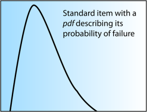
Traditionally in a reliability block diagram, one assumes independence and thus an item's failure characteristics can be fully described by its failure distribution. However, if the configuration includes load sharing redundancy, then a single failure distribution is no longer sufficient to describe an item's failure characteristics. Instead, the item will fail differently when operating under different loads and the load applied to the component will vary depending on the performance of the other component(s) in the configuration. Therefore, a more complex model is needed to fully describe the failure characteristics of such blocks. This model must describe both the effect of the load (or stress) on the life of the product and the probability of failure of the item at the specified load. The models, theory and methodology used in Quantitative Accelerated Life Testing (QALT) data analysis can be used to obtain the desired model for this situation. The objective of QALT analysis is to relate the applied stress to life (or a life distribution). Identically in the load sharing case, one again wants to relate the applied stress (or load) to life. The following figure graphically illustrates the probability density function (pdf) for a standard item, where only a single distribution is required.
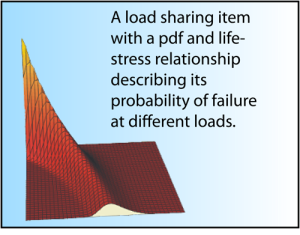
The next figure represents a load sharing item by using a 3-D surface that illustrates the pdf , load and time.
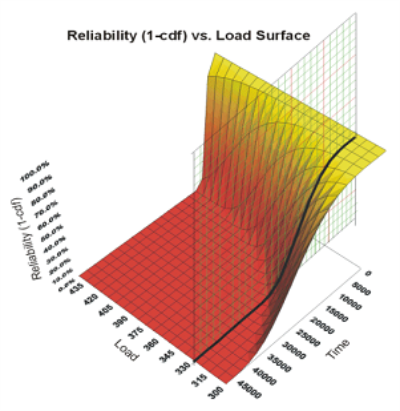
The following figure shows the reliability curve for a load sharing item vs. the applied load.
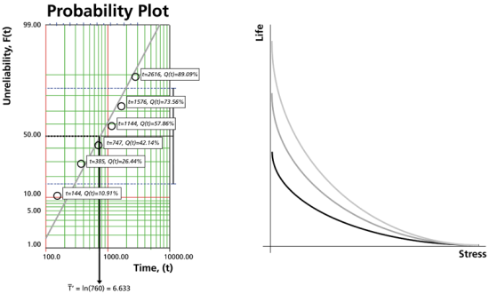
To formulate the model, a life distribution is combined with a life-stress relationship. The distribution choice is based on the product's failure characteristics while the life-stress relationship is based on how the stress affects the life characteristics. The following figure graphically shows these elements of the formulation.
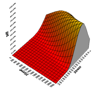
The next figure shows the combination of both an underlying distribution and a life-stress model by plotting a pdf against both time and stress.
The assumed underlying life distribution can be any life distribution. The most commonly used life distributions include the Weibull, the exponential and the lognormal. The life-stress relationship describes how a specific life characteristic changes with the application of stress. The life characteristic can be any life measure such as the mean, median,
,
, etc. It is expressed as a function of stress. Depending on the assumed underlying life distribution, different life characteristics are considered. Typical life characteristics for some distributions are shown in the next table.
| Distribution | Parameters | Life Characteristic |
|---|---|---|
| Weibull | Scale parameter, |
|
| Exponential | Mean Life, ( |
|
| Lognormal | Median, |
|
| *Usually assumed constant | ||
For example, when considering the Weibull distribution, the scale parameter,
, is chosen to be the life characteristic that is stress-dependent while
is assumed to remain constant across different stress levels. A life-stress relationship is then assigned to
For a detailed discussion of this topic, see ReliaSoft's Accelerated Life Testing Data Analysis Reference.


![{\displaystyle P\left[{\underset {i=1}{\overset {n}{\mathop {\bigcap } }}}\,{{A}_{i}}\right]={\underset {i=1}{\overset {n}{\mathop {\prod } }}}\,P({{A}_{i}})\ \,\!}](https://en.wikipedia.org/api/rest_v1/media/math/render/svg/14694bf9f9b3bed22fda6ef3dd2631c12d5e4907)


![{\displaystyle [a,b]\,\!}](https://en.wikipedia.org/api/rest_v1/media/math/render/svg/08268f073d76e500a09a309a45bcc9f19e599db4)


![{\displaystyle [0,+\infty ].\,\!}](https://en.wikipedia.org/api/rest_v1/media/math/render/svg/c915ac889d2ae78a7fa45708ed0f96b105471636)


![{\displaystyle {\frac {d\left[f(t)\right]}{dt}}=0\ \,\!}](https://en.wikipedia.org/api/rest_v1/media/math/render/svg/d8059c99393d6b91d82de8d1b03069ce99bd1d7b)


