Introduction to Repairable Systems
In prior chapters, the analysis was focused on determining the reliability of the system (i.e., the probability that the system, subsystem or component will operate successfully by a given time,
. The prior formulations provided us with the probability of success of the entire system, up to a point in time, without looking at the question: "What happens if a component fails during that time and is then fixed?" In dealing with repairable systems, these definitions need to be redefined and adapted to deal with this case of the renewal of systems/components.
Repairable systems receive maintenance actions that restore/renew system components when they fail. These actions change the overall makeup of the system. These actions must now be taken into consideration when assessing the behavior of the system because the age of the system components is no longer uniform nor is the time of operation of the system continuous.
In attempting to understand the system behavior, additional information and models are now needed for each system component. Our primary input in the prior chapters was a model that described how the component failed (its failure probability distribution). When dealing with components that are repaired, one also needs to know how long it takes for the component to be restored. That is, at the very least, one needs a model that describes how the component is restored (a repair probability distribution).
In this chapter, we will introduce the additional information, models and metrics required to fully analyze a repairable system.
Defining Maintenance
To properly deal with repairable systems, we need to first understand how components in these systems are restored (i.e., the maintenance actions that the components undergo). In general, maintenance is defined as any action that restores failed units to an operational condition or retains non-failed units in an operational state. For repairable systems, maintenance plays a vital role in the life of a system. It affects the system's overall reliability, availability, downtime, cost of operation, etc. Generally, maintenance actions can be divided into three types: corrective maintenance, preventive maintenance and inspections.
Corrective Maintenance
Corrective maintenance consists of the action(s) taken to restore a failed system to operational status. This usually involves replacing or repairing the component that is responsible for the failure of the overall system. Corrective maintenance is performed at unpredictable intervals because a component's failure time is not known a priori. The objective of corrective maintenance is to restore the system to satisfactory operation within the shortest possible time. Corrective maintenance is typically carried out in three steps:
- Diagnosis of the problem. The maintenance technician must take time to locate the failed parts or otherwise satisfactorily assess the cause of the system failure.
- Repair and/or replacement of faulty component(s). Once the cause of system failure has been determined, action must be taken to address the cause, usually by replacing or repairing the components that caused the system to fail.
- Verification of the repair action. Once the components in question have been repaired or replaced, the maintenance technician must verify that the system is again successfully operating.
Preventive Maintenance
Preventive maintenance, unlike corrective maintenance, is the practice of replacing components or subsystems before they fail in order to promote continuous system operation. The schedule for preventive maintenance is based on observation of past system behavior, component wear-out mechanisms and knowledge of which components are vital to continued system operation. Cost is always a factor in the scheduling of preventive maintenance. In many circumstances, it is financially more sensible to replace parts or components that have not failed at predetermined intervals rather than to wait for a system failure that may result in a costly disruption in operations. Preventive maintenance scheduling strategies are discussed in more detail later in this chapter.
Inspections
Inspections are used in order to uncover hidden failures (also called dormant failures). In general, no maintenance action is performed on the component during an inspection unless the component is found failed, in which case a corrective maintenance action is initiated. However, there might be cases where a partial restoration of the inspected item would be performed during an inspection. For example, when checking the motor oil in a car between scheduled oil changes, one might occasionally add some oil in order to keep it at a constant level. The subject of inspections is discussed in more detail in Repairable Systems Analysis Through Simulation.
Downtime Distributions
Maintenance actions (preventive or corrective) are not instantaneous. There is a time associated with each action (i.e., the amount of time it takes to complete the action). This time is usually referred to as downtime and it is defined as the length of time an item is not operational. There are a number of different factors that can affect the length of downtime, such as the physical characteristics of the system, spare part availability, repair crew availability, human factors, environmental factors, etc. Downtime can be divided into two categories based on these factors:
- Waiting Downtime. This is the time during which the equipment is inoperable but not yet undergoing repair. This could be due to the time it takes for replacement parts to be shipped, administrative processing time, etc.
- Active Downtime. This is the time during which the equipment is inoperable and actually undergoing repair. In other words, the active downtime is the time it takes repair personnel to perform a repair or replacement. The length of the active downtime is greatly dependent on human factors, as well as on the design of the equipment. For example, the ease of accessibility of components in a system has a direct effect on the active downtime.
These downtime definitions are subjective and not necessarily mutually exclusive nor all-inclusive. As an example, consider the time required to diagnose the problem. One may need to diagnose the problem before ordering parts and then wait for the parts to arrive.
The influence of a variety of different factors on downtime results in the fact that the time it takes to repair/restore a specific item is not generally constant. That is, the time-to-repair is a random variable, much like the time-to-failure. The statement that it takes on average five hours to repair implies an underlying probabilistic distribution. Distributions that describe the time-to-repair are called repair distributions (or downtime distributions) in order to distinguish them from the failure distributions. However, the methods employed to quantify these distributions are not any different mathematically than the methods employed to quantify failure distributions. The difference is in how they are employed (i.e., the events they describe and metrics used). As an example, when using a life distribution with failure data (i.e., the event modeled was time-to-failure), unreliability provides the probability that the event (failure) will occur by that time, while reliability provides the probability that the event (failure) will not occur. In the case of downtime distributions, the data set consists of times-to-repair, thus what we termed as unreliability now becomes the probability of the event occurring (i.e., repairing the component). Using these definitions, the probability of repairing the component by a given time,
, is also called the component's maintainability.
Maintainability
Maintainability is defined as the probability of performing a successful repair action within a given time. In other words, maintainability measures the ease and speed with which a system can be restored to operational status after a failure occurs. For example, if it is said that a particular component has a 90% maintainability in one hour, this means that there is a 90% probability that the component will be repaired within an hour. In maintainability, the random variable is time-to-repair, in the same manner as time-to-failure is the random variable in reliability. As an example, consider the maintainability equation for a system in which the repair times are distributed exponentially. Its maintainability
is given by:
where = repair rate.
Note the similarity between this equation and the equation for the reliability of a system with exponentially distributed failure times. However, since the maintainability represents the probability of an event occurring (repairing the system) while the reliability represents the probability of an event not occurring (failure), the maintainability expression is the equivalent of the unreliability expression,
. Furthermore, the single model parameter
is now referred to as the repair rate, which is analogous to the failure rate,
, used in reliability for an exponential distribution.
Similarly, the mean of the distribution can be obtained by:
This now becomes the mean time to repair (
) instead of the mean time to failure (
).
The same concept can be expanded to other distributions. In the case of the Weibull distribution, maintainability,
, is given by:
While the mean time to repair ( ) is given by:
And the Weibull repair rate is given by:
As a last example, if a lognormal distribution is chosen, then:
where:
-
mean of the natural logarithms of the times-to-repair.
standard deviation of the natural logarithms of the times-to-repair.
It should be clear by now that any distribution can be used, as well as related concepts and methods used in life data analysis, the only difference being that instead of times-to-failure we are using times-to-repair. What one chooses to include in the time-to-repair varies, but can include:
- The time it takes to successfully diagnose the cause of the failure.
- The time it takes to procure or deliver the parts necessary to perform the repair.
- The time it takes to gain access to the failed part or parts.
- The time it takes to remove the failed components and replace them with functioning ones.
- The time involved with bringing the system back to operating status.
- The time it takes to verify that the system is functioning within specifications.
- The time associated with closing up a system and returning it to normal operation.
In the interest of being fair and accurate, one should disclose (document) what was and was not included in determining the repair distribution.
Availability
If one considers both reliability (probability that the item will not fail) and maintainability (the probability that the item is successfully restored after failure), then an additional metric is needed for the probability that the component/system is operational at a given time,
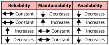
(i.e., has not failed or it has been restored after failure). This metric is availability. Availability is a performance criterion for repairable systems that accounts for both the reliability and maintainability properties of a component or system. It is defined as the probability that the system is operating properly when it is requested for use. That is, availability is the probability that a system is not failed or undergoing a repair action when it needs to be used. For example, if a lamp has a 99.9% availability, there will be one time out of a thousand that someone needs to use the lamp and finds out that the lamp is not operational either because the lamp is burned out or the lamp is in the process of being replaced. Note that this metric alone tells us nothing about how many times the lamp has been replaced. For all we know, the lamp may be replaced every day or it could have never been replaced at all. Other metrics are still important and needed, such as the lamp's reliability. The next table illustrates the relationship between reliability, maintainability and availability.
A Brief Introduction to Renewal Theory
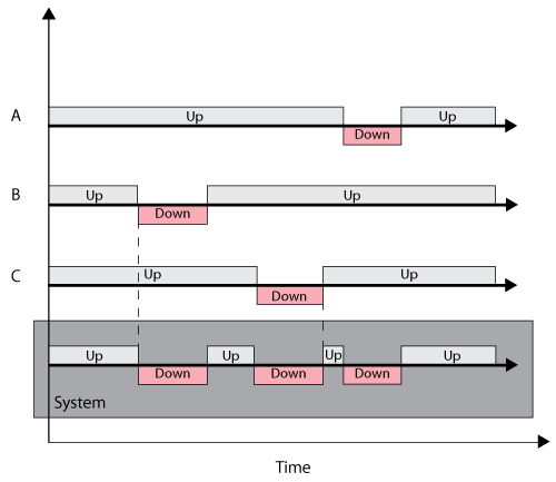
For a repairable system, the time of operation is not continuous. In other words, its life cycle can be described by a sequence of up and down states. The system operates until it fails, then it is repaired and returned to its original operating state. It will fail again after some random time of operation, get repaired again, and this process of failure and repair will repeat. This is called a renewal process and is defined as a sequence of independent and non-negative random variables. In this case, the random variables are the times-to-failure and the times-to-repair/restore. Each time a unit fails and is restored to working order, a renewal is said to have occurred. This type of renewal process is known as an alternating renewal process because the state of the component alternates between a functioning state and a repair state, as illustrated in the following graphic.

A system's renewal process is determined by the renewal processes of its components. For example, consider a series system of three statistically independent components. Each component has a failure distribution and a repair distribution. Since the components are in series, when one component fails, the entire system fails. The system is then down for as long as the failed component is under repair. The following figure illustrates this.
One of the main assumptions in renewal theory is that the failed components are replaced with new ones or are repaired so they are as good as new, hence the name renewal. One can make the argument that this is the case for every repair, if you define the system in enough detail. In other words, if the repair of a single circuit board in the system involves the replacement of a single transistor in the offending circuit board, then if the analysis (or RBD) is performed down to the transistor level, the transistor itself gets renewed. In cases where the analysis is done at a higher level, or if the offending component is replaced with a used component, additional steps are required. We will discuss this in later chapters using a restoration factor in the analysis. For more details on renewal theory, interested readers can refer to Elsayed [7] and Leemis [17].
Availability Classifications
The definition of availability is somewhat flexible and is largely based on what types of downtimes one chooses to consider in the analysis. As a result, there are a number of different classifications of availability, such as:
Instantaneous or Point Availability,
Instantaneous (or point) availability is the probability that a system (or component) will be operational (up and running) at any random time, t. This is very similar to the reliability function in that it gives a probability that a system will function at the given time, t. Unlike reliability, the instantaneous availability measure incorporates maintainability information. At any given time, t, the system will be operational if the following conditions are met Elsayed ([7]):
The item functioned properly from to
with probability
or it functioned properly since the last repair at time u,
, with probability:
With being the renewal density function of the system.
Then the point availability is the summation of these two probabilities, or:
Average Uptime Availability (or Mean Availability),
The mean availability is the proportion of time during a mission or time period that the system is available for use. It represents the mean value of the instantaneous availability function over the period (0, T] and is given by:
Steady State Availability,
The steady state availability of the system is the limit of the instantaneous availability function as time approaches infinity or:
The figure shown next also graphically illustrates this.
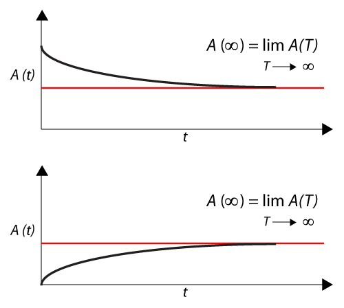
In other words, one can think of the steady state availability as a stabilizing point where the system's availability is a constant value. However, one has to be very careful in using the steady state availability as the sole metric for some systems, especially systems that do not need regular maintenance. A large scale system with repeated repairs, such as a car, will reach a point where it is almost certain that something will break and need repair once a month. However, this state may not be reached until, say, 500,000 miles. Obviously, if I am an operator of rental vehicles and I only keep the vehicles until they reach 50,000 miles, then this value would not be of any use to me. Similarly, if I am an auto maker and only warrant the vehicles to
miles, is knowing the steady state value useful?
Inherent Availability,
Inherent availability is the steady state availability when considering only the corrective downtime of the system.
For a single component, this can be computed by:
This gets slightly more complicated for a system. To do this, one needs to look at the mean time between failures, or
, and compute this as follows:
This may look simple. However, one should keep in mind that until the steady state is reached, the
may be a function of time (e.g., a degrading system), thus the above formulation should be used cautiously. Furthermore, it is important to note that the
defined here is different from the
(or more precisely for a repairable system,
, mean time to first failure).
Achieved Availability,
Achieved availability is very similar to inherent availability with the exception that preventive maintenance (PM) downtimes are also included. Specifically, it is the steady state availability when considering corrective and preventive downtime of the system. It can be computed by looking at the mean time between maintenance actions,
and the mean maintenance downtime,
or:
Operational Availability,
Operational availability is a measure of the average availability over a period of time and it includes all experienced sources of downtime, such as administrative downtime, logistic downtime, etc.
Operational availability is the ratio of the system uptime and total time. Mathematically, it is given by:
Where the operating cycle is the overall time period of operation being investigated and uptime is the total time the system was functioning during the operating cycle.
When there is no specified logistic downtime or preventive maintenance, the above equation returns the Mean Availability of the system. The operational availability is the availability that the customer actually experiences. It is essentially the a posteriori availability based on actual events that happened to the system. The previous availability definitions are a priori estimations based on models of the system failure and downtime distributions. In many cases, operational availability cannot be controlled by the manufacturer due to variation in location, resources and other factors that are the sole province of the end user of the product.
Example: Calculating Availability
As an example, consider the following scenario. A diesel power generator is supplying electricity at a research site in Antarctica. The personnel are not satisfied with the generator. They estimated that in the past six months, they were without electricity due to generator failure for an accumulated time of 1.5 months. Therefore, the operational availability of the diesel generator experienced by the personnel of the station is:
Obviously, this is not satisfactory performance for an electrical generator in such a climate, so alternatives to this source of electricity are investigated. One alternative under consideration is a wind-powered electrical turbine, which the manufacturer claims to have a 99.71% availability. This is much higher than the availability experienced by the crew of the Antarctic research station for the diesel generator. Upon investigation, it was found that the wind-turbine manufacturer estimated the availability based on the following information:
| Failure Distribution | Repair Distribution |
|---|---|
| Exponential, |
Exponential, |
Based on the above information, one can estimate the mean availability for the wind turbine over a period of six months to be:
This availability, however, was obtained solely by considering the claimed failure and repair properties of the wind-turbine. Waiting downtime was not considered in the above calculation. Therefore, this availability measure cannot be compared to the operational availability for the diesel generator since the two availability measurements have different inputs. This form of availability measure is also known as inherent availability. In order to make a meaningful comparison, the inherent availability of the diesel generator needs to be estimated. The diesel generator has an
= 50 days (or 1200 hours) and an
= 3 hours. Thus, an estimate of the mean availability is:
Note that the inherent availability of the diesel generator is actually a little bit better than the inherent availability of the wind-turbine! Even though the diesel generator has a higher failure rate, its mean-time-to-repair is much smaller than that of the wind turbine, resulting in a slightly higher inherent availability value. This example illustrates the potentially large differences in the types of availability measurements, as well as their misuse. In this example, the operational availability is much lower than the inherent availability. This is because the inherent availability does not account for downtime due to administrative time, logistic time, the time required to obtain spare parts or the time it takes for the repair personnel to arrive at the site.
Preventive Maintenance
Preventive maintenance (PM) is a schedule of planned maintenance actions aimed at the prevention of breakdowns and failures. The primary goal of preventive maintenance is to prevent the failure of equipment before it actually occurs. It is designed to preserve and enhance equipment reliability by replacing worn components before they actually fail. Preventive maintenance activities include equipment checks, partial or complete overhauls at specified periods, oil changes, lubrication and so on. In addition, workers can record equipment deterioration so they know to replace or repair worn parts before they cause system failure. Recent technological advances in tools for inspection and diagnosis have enabled even more accurate and effective equipment maintenance. The ideal preventive maintenance program would prevent all equipment failure before it occurs.
Value of Preventive Maintenance
There are multiple misconceptions about preventive maintenance. One such misconception is that PM is unduly costly. This logic dictates that it would cost more for regularly scheduled downtime and maintenance than it would normally cost to operate equipment until repair is absolutely necessary. This may be true for some components; however, one should compare not only the costs but the long-term benefits and savings associated with preventive maintenance. Without preventive maintenance, for example, costs for lost production time from unscheduled equipment breakdown will be incurred. Also, preventive maintenance will result in savings due to an increase of effective system service life.
Long-term benefits of preventive maintenance include:
- Improved system reliability.
- Decreased cost of replacement.
- Decreased system downtime.
- Better spares inventory management.
Long-term effects and cost comparisons usually favor preventive maintenance over performing maintenance actions only when the system fails.
When Does Preventive Maintenance Make Sense?
Preventive maintenance is a logical choice if, and only if, the following two conditions are met:
- Condition #1: The component in question has an increasing failure rate. In other words, the failure rate of the component increases with time, implying wear-out. Preventive maintenance of a component that is assumed to have an exponential distribution (which implies a constant failure rate) does not make sense!
- Condition #2: The overall cost of the preventive maintenance action must be less than the overall cost of a corrective action.
If both of these conditions are met, then preventive maintenance makes sense. Additionally, based on the costs ratios, an optimum time for such action can be easily computed for a single component. This is detailed in later sections.
The Fallacy of "Constant Failure Rate" and "Preventive Replacement"
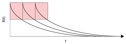
Even though we alluded to the fact in the last section, it is important to make it explicitly clear that if a component has a constant failure rate (i.e., defined by an exponential distribution), then preventive maintenance of the component will have no effect on the component's failure occurrences. To illustrate this, consider a component with an
=
hours, or
, and with preventive replacement every 50 hours. The reliability vs. time graph for this case is illustrated in the following figure, where the component is replaced every 50 hours, thereby resetting the component's reliability to one. At first glance, it may seem that the preventive maintenance action is actually maintaining the component at a higher reliability.
However, consider the following cases for a single component:
Case 1: The component's reliability from 0 to 60 hours:
- With preventive maintenance, the component was replaced with a new one at 50 hours so the overall reliability is based on the reliability of the new component for 10 hours,
, times the reliability of the previous component,
. The result is
- Without preventive maintenance, the reliability would be the reliability of the same component operating to 60 hours, or
.
Case 2: The component's reliability from 50 to 60 hours:
- With preventive maintenance, the component was replaced at 50 hours, so this is solely based on the reliability of the new component for a mission of 10 hours, or
.
- Without preventive maintenance, the reliability would be the conditional reliability of the same component operating to 60 hours, having already survived to 50 hours, or
.
As can be seen, both cases —with and without preventive maintenance—yield the same results.
Determining Preventive Replacement Time
As mentioned earlier, if the component has an increasing failure rate, then a carefully designed preventive maintenance program is beneficial to system availability. Otherwise, the costs of preventive maintenance might actually outweigh the benefits. The objective of a good preventive maintenance program is to either minimize the overall costs (or downtime, etc.) or meet a reliability objective. In order to achieve this, an appropriate interval (time) for scheduled maintenance must be determined. One way to do that is to use the optimum age replacement model, as presented next. The model adheres to the conditions discussed previously:
- The component is exhibiting behavior associated with a wear-out mode. That is, the failure rate of the component is increasing with time.
- The cost for planned replacements is significantly less than the cost for unplanned replacements.
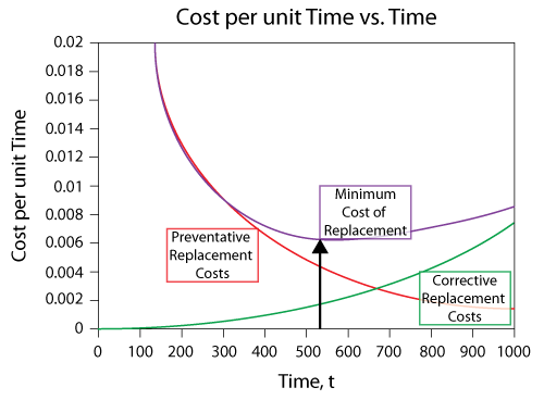
The following figure shows the Cost Per Unit Time vs. Time plot and it can be seen that the corrective replacement costs increase as the replacement interval increases. In other words, the less often you perform a PM action, the higher your corrective costs will be. Obviously, as we let a component operate for longer times, its failure rate increases to a point that it is more likely to fail, thus requiring more corrective actions. The opposite is true for the preventive replacement costs. The longer you wait to perform a PM, the less the costs; if you do PM too often, the costs increase. If we combine both costs, we can see that there is an optimum point that minimizes the costs. In other words, one must strike a balance between the risk (costs) associated with a failure while maximizing the time between PM actions.
Optimum Age Replacement Policy
To determine the optimum time for such a preventive maintenance action (replacement), we need to mathematically formulate a model that describes the associated costs and risks. In developing the model, it is assumed that if the unit fails before time
, a corrective action will occur and if it does not fail by time
, a preventive action will occur. In other words, the unit is replaced upon failure or after a time of operation,
, whichever occurs first.
Thus, the optimum replacement time can be found by minimizing the cost per unit time,
is given by:
where:
-
= reliability at time
.
= cost of planned replacement.
= cost of unplanned replacement.
The optimum replacement time interval,
, is the time that minimizes
This can be found by solving for
such that:
Or by solving for a that satisfies the following equation:
Interested readers can refer to Barlow and Hunter [2] for more details on this model.
In BlockSim (Version 8 and above), you can use the Optimum Replacement window to determine the optimum replacement time either for an individual block or for multiple blocks in a diagram simultaneously. When working with multiple blocks, the calculations can be for individual blocks or for one or more groups of blocks. For each item that is included in the optimization calculations, you will need to specify the cost for a planned replacement and the cost for an unplanned replacement. This is done by calculating the costs for replacement based on the item settings using equations or simulation and then, if desired, manually entering any additional costs for either type of replacement in the corresponding columns of the table.
The equations used to calculate the costs of planned and unplanned tasks for each item based on its associated URD are as follows:
- For the cost of planned tasks, here denoted as PM cost:
- Only PM tasks based on item age or system age (fixed or dynamic intervals) are considered. If there is more than one PM task based on item age, only the first one is considered.
- For the cost of the unplanned task, here denoted as CM cost:
When using simulation, for costs associated with planned replacements, all preventive tasks based on item age or system age (fixed or dynamic intervals) are considered. Because each item is simulated as a system (i.e., in isolation from any other item), tasks triggered in other ways are not considered.
Example: Optimum Replacement Time
The failure distribution of a component is described by a 2-parameter Weibull distribution with
and
hours.
- The cost for a corrective replacement is $5.
- The cost for a preventive replacement is $1.
Estimate the optimum replacement age in order to minimize these costs.
Solution
Prior to obtaining an optimum replacement interval for this component, the assumptions of the following equation must be checked.
The component has an increasing failure rate because it follows a Weibull distribution with
greater than 1. Note that if
, then the component has a constant failure rate, but if
, then it has a decreasing failure rate. If either of these cases exist, then preventive replacement is unwise. Furthermore, the cost for preventive replacement is less than the corrective replacement cost. Thus, the conditions for the optimum age replacement policy have been met.
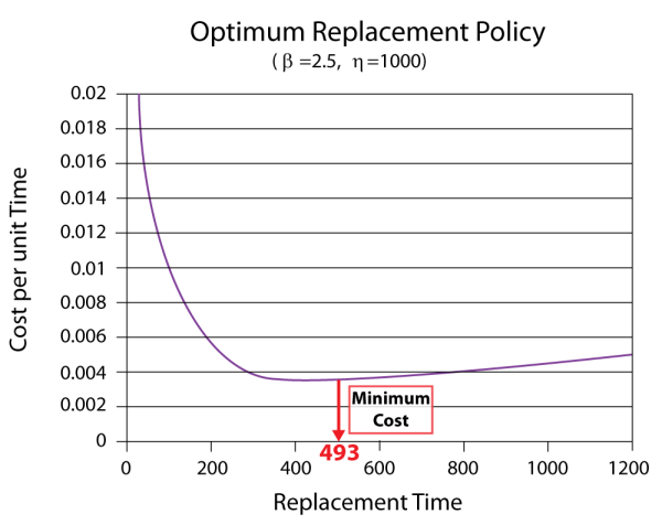
Using BlockSim, enter the parameters of the Weibull distribution in the component's Block Properties window. Next, open the Optimum Replacement window and enter the 1 in the Planned Replacement Cost column, and 5 in the Unplanned Replacement Cost column. Click Calculate. In the Optimum Replacement Calculations window that appears, select the Individual option and click OK. The optimum replacement time for the component is estimated to be 493.0470, as shown next.

The figure below shows the Cost vs. Time plot of the component (with the scaling adjusted and the plot annotated to show the minimum cost).
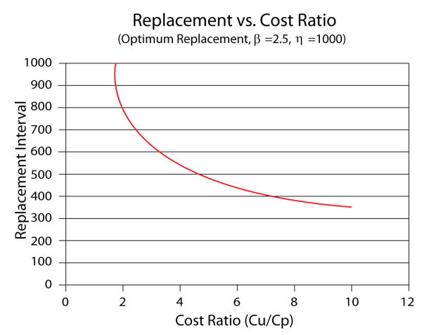
If we enter different cost values in the Unplanned Replacement Cost column and obtain the optimum replacement time at each value, we can use the data points to create a plot that shows the effect of the corrective cost on the optimum replacement interval. The following plot shows an example. In this case, the optimum replacement interval decreases as the cost ratio increases. This is an expected result because the corrective replacement costs are much greater than the preventive replacement costs. Therefore, it is more cost-effective to replace the component more frequently before it fails.
Applying These Principles to Larger Systems
In this chapter, we explored some of the basic concepts and mathematical formulations involving repairable systems. Most examples/equations were given using a single component and, in some cases, using the exponential distribution for simplicity. In practical applications where one is dealing with large systems composed of many components that fail and get repaired based on different distributions and with additional constraints (such as spare parts, crews, etc.), exact analytical computations become intractable. To solve such systems, one needs to resort to simulation (more specifically, discrete event simulation) to obtain the metrics/results discussed in this section. Repairable Systems Analysis Through Simulation expands on these concepts and introduces these simulation methods.


![{\displaystyle {\begin{aligned}CPUT\left(t\right)=&{\frac {\text{Total Expected Replacement Cost per Cycle}}{\text{Expected Cycle Length}}}\\=&{\frac {{{C}_{P}}\cdot R\left(t\right)+{{C}_{U}}\cdot \left[1-R\left(t\right)\right]}{\int _{0}^{t}R\left(s\right)ds}}\end{aligned}}\,\!}](https://en.wikipedia.org/api/rest_v1/media/math/render/svg/235f8454611d8482cfeb3707396763c6ef0a3859)


![{\displaystyle {\frac {\partial \left[CPUT(t)\right]}{\partial t}}=0\,\!}](https://en.wikipedia.org/api/rest_v1/media/math/render/svg/313eee8c07f2fdea19477cb35a3eae5d902ee874)
![{\displaystyle {\frac {\partial \left[{\tfrac {{{C}_{P}}\cdot R\left(t\right)+{{C}_{U}}\cdot \left[1-R\left(t\right)\right]}{\int _{0}^{t}R\left(s\right)ds}}\right]}{\partial t}}=0\,\!}](https://en.wikipedia.org/api/rest_v1/media/math/render/svg/adc46334e85ea1b2a18389546e60bca7ebd3bc3f)


