Discrete Markov Diagrams

In discrete Markov diagrams, the system moves from state to state in steps. These steps are not necessarily time-based; although they can represent a fixed period of time, they can also represent distance or any other measurement. At each step, there is a fixed probability of the system transitioning to another state.

This topic describes how to create a discrete Markov diagram that is ready for analysis. For information about analysis results, see Markov Diagram Results and Markov Diagram Plots.

Define the States

Add a state block to represent each state that the system can be in.

To configure a state block in a discrete Markov diagram, you will need to specify the probability that the system will be in that state during the first step of the analysis in the Initial Probability field. The sum of the initial probability values for all of the state blocks in the diagram must be equal to 1.

The state block may be configured to store the mean probability of the state at the end of the analysis in a variable. The Storage Variable field displays the name of the variable, if any.

Define the Transitions

Connect the state blocks in the diagram to show the possible transitions between states. Once you have drawn each transition, double-click it to open the Transition Properties window. Define the probability of the system moving from the source state to the target state by assigning a constant model for the Transition Probability.

For any state, the sum of the probabilities of the outgoing transitions must be less than or equal to 1. If it is less than 1, the probability of the system remaining in the state is equal to (1 - the sum of the probabilities of the outgoing transitions).

Note that if a state does not have any outgoing transitions, then once the system enters that state, it cannot leave it. This kind of state is called a sink.

Specify the Analysis Length

In the Number of Steps field on the control panel, specify the number of steps to be performed when analyzing the diagram. At each step, the probability of being in a particular state is calculated based on the current probability of being in a particular state and the specified transition probability values. After a certain number of steps, the diagram will reach a steady state, meaning that calculations beyond that point offer no additional information.

Discrete Markov Diagram Example

To demonstrate the use of discrete Markov diagrams with a very simple example, let's assume that a day can be either sunny or rainy, and that today is sunny. You want to look at the chances of sun and rain for the next 20 days.

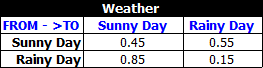
When a day is sunny, there is a 55% chance that the next day will be rainy and a 45% chance that the next day will be sunny. When a day is rainy, there is an 85% chance that the next day will be sunny and a 15% chance that the next day will be rainy. This can be represented by the following transition matrix:

You create a discrete Markov diagram and add the following:

• A state block called "Sunny Day" with an initial probability value of 1. This reflects the fact that today is sunny (i.e., there is a 100% chance of a sunny day).
• A state block called "Rainy Day" with an initial probability of 0.

You then connect the blocks. For the transition from "Sunny Day" to "Rainy Day," you use a constant model equal to 0.55. For the transition from "Rainy Day" to "Sunny Day," you use a constant model equal to 0.85.

The Markov diagram is shown next, with all associated block and transition properties windows.

Note that when it is a sunny day, the probability of it remaining in that state the next day is 0.45 (1.00 - the 0.55 probability of a rainy day), as shown at the upper left corner of the "Sunny Day" block. Similarly, when it is a rainy day, the probability of the next day being rainy is 0.15 (1.00 - 0.85), as shown for the "Rainy Day" block.

You then click the Diagram Properties icon on the control panel and enter 20 in the Length (Steps) field. Then you click Calculate to analyze the diagram.

A variety of results will be available in the plot sheet, QCP and Results Explorer.

For example, you click Show Results to open the explorer.

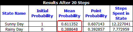
On the Result Summary page, you can see that the mean probability of the system being in the "Sunny Day" state is approximately 0.611, and the mean probability of the system being in the "Rainy Day" state is approximately 0.389, as shown next.