Continuous Markov Diagrams
In continuous Markov diagrams, the system does not proceed according to fixed steps. Instead, the rates at which the system's states transition are determined from exponential distributions.
This topic describes how to create a continuous Markov diagram that is ready for analysis. For information about analysis results, see Markov Diagram Results and Markov Diagram Plots.
Define the States
Add a state block to represent each state that the system can be in.
To configure a state block in a continuous Markov diagram, you will need to specify the following:
- In the State Type field, specify whether the system is available or unavailable when in that state. Unavailable states are indicated within the diagram by a red triangle at the lower right corner of the block.
- In the Initial Probability field, enter the probability that the system will be in that state at time equal to 0. The sum of the initial probability values for all of the state blocks in the diagram must be equal to 1.
- In the Cost field, enter the cost per unit time, if any, associated with the system being in that state. Note that you can specify a negative cost, which is a profit.
The state block may be configured to store the mean availability of that state at the end of the analysis in a variable. The Storage Variable field displays the name of the variable, if any.
Define the Transitions
Connect the state blocks in the diagram to show the possible transitions between states. Once you have drawn each transition, double-click it to open the Transition Properties window. Assign a 1-parameter exponential model for the Transition Probability. This model represents the time at which the system moves from the source state to the target state.
Note that if a state does not have any outgoing transitions, then once the system enters that state, it cannot leave it. This kind of state is called a sink.
Specify the Analysis Length
In the Operating Time field on the control panel, specify the length of time to be considered when analyzing the diagram.
Continuous Markov Diagram Example
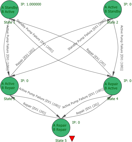
To demonstrate the use of continuous Markov diagrams with a very simple example, let's assume that you have a system with two pumps, A and B. At any given time, the system may be in one of 5 states:
- B is active, A is in standby. Both are in working condition. This is the state in which you want analysis to start.
- A is active, B is in standby. Both are in working condition.
- B fails. A is active and B is undergoing repair.
- A fails. B is active while A is undergoing repair.
- Both pumps are undergoing repair.
A pump that is active fails according to a 1-parameter exponential distribution with a mean time of 100 hours. A pump that is in standby fails according to a 1-parameter exponential distribution with a mean time of 200 hours. Repair time is described by a 1-parameter exponential distribution with a mean time of 20 hours.
You create a continuous Markov diagram and add the following:
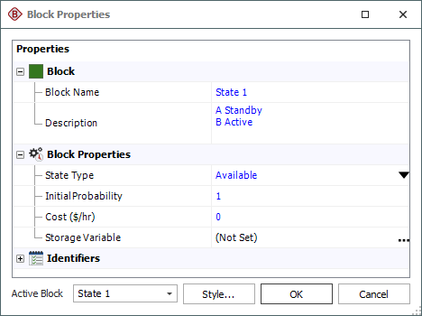
- A state block called "State 1" with an initial probability value of 1 and a state type of available.
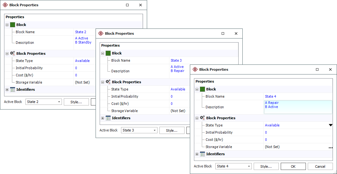
- 3 state blocks, "State 2," "State 3" and "State 4," each with an initial probability value of 0 and a state type of available.
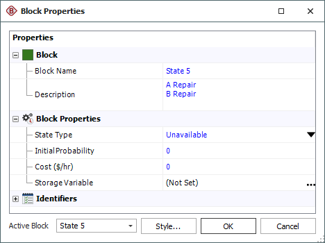
- A state block called "State 5" with an initial probability value of 0 and a state type of unavailable.
You then create models to represent the failure rate of active pumps, the failure rate of standby pumps and the repair time. You use these models to define the state transitions. The Markov diagram is shown next.
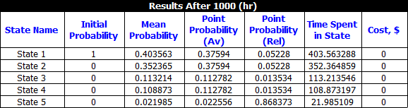
The Result Summary table is shown next.