Phases in Markov Diagrams

In much the same way that you can use phase diagrams to represent systems that change over time, you can use phases in Markov diagrams to represent situations where the transitions between states change over time.

To enable phases in any Markov diagram, select the Use phases check box in the control panel. The Phases panel will appear at the bottom of the diagram, and the current diagram will be shown as Phase 1 in the panel.

To add another phase, click the Add Phase icon in the Phase panel.

A new phase will be added to the end of the phase list. Each new phase is created as a copy of the phase that is currently selected in the Phase panel; you can then edit the phase as desired. The panel shows a thumbnail of each phase. To see a larger view of any phase that is not currently selected, move the pointer over the thumbnail.

To delete a phase, select it in the Phase panel and click the Delete Phase icon.

The order in which the phases are shown in the Phase panel dictates the order in which they will be performed during analysis. You can change the order of the phases by clicking the Phase Order icon.

To change the phase name or specify how long the phase will run (number of steps for a discrete diagram, length of time for a continuous diagram), click the Phase Properties icon.

Specifying the Analysis Length

The total length of the analysis is, by default, equal to the sum of the lengths of all phases; this is considered to be "one cycle." For example, if you are working with a continuous Markov diagram that has 3 phases, where Phase 1 has a duration of 100 hours, Phase 2 has a duration of 50 hours and Phase 3 has a duration of 25 hours, then one cycle for the analysis will be 175 hours.

You can change the analysis length by specifying a new Operating Time (for continuous diagrams) or Number of Steps (for discrete diagrams) on the control panel. For instance, in the case mentioned here, if you specify an operating time of 200 hours, then Phase 1 will run for 100 hours, Phase 2 for 50 hours, Phase 3 for 25 hours and then Phase 1 will run again for the remaining 25 hours.

For continuous diagrams, if the analysis length that you have specified is not equal to one cycle, you can reset the value to one cycle by clicking the Set to One Cycle icon.

Example: Phases in Markov Diagrams

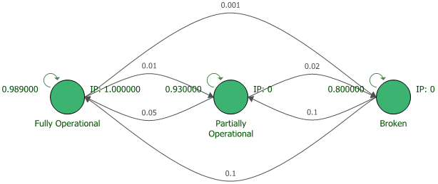
To demonstrate the use of phases in Markov diagrams with a very simple example, consider a case where a system is made up of a compressor. Initially, the compressor is fully operational. During normal operating conditions, after each usage cycle:

• If the compressor is fully operational, there is a 1% chance that it degrades to only partially operational and a 0.1% chance that it breaks completely.
• If the compressor is partially operational, there is a 2% chance that it breaks and a 5% chance that it is repaired to fully operational status.
• If the compressor is broken, there is a 10% chance that it is repaired only to partially operational status and a 10% chance that it is repaired to fully operational status.

The transition matrix and discrete Markov diagram for this look like this:

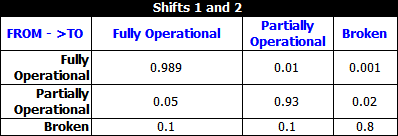
Let’s assume that the compressor runs in an environment where there are three shifts, and completes 10 usage cycles during each shift. During the third shift, nobody is available to perform repairs. This means that during those hours, the transition matrix and Markov diagram look instead like this:

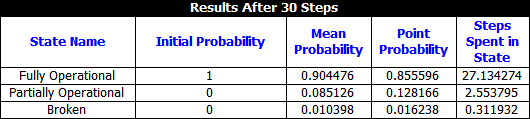
This is easily modeled with two phases. The “Shifts 1 and 2” phase runs for 20 usage cycles and the “Shift 3” phase runs for 10 usage cycles; the total analysis length is 30 usage cycles.

The result summary for the analysis is shown next.

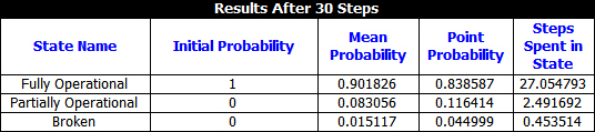
Compare this to the following result summary, which shows the values for an analysis of 30 usage cycles where all three shifts have repair personnel available.