Contour Plots and Confidence Bounds on Parameters

There are multiple ways to estimate the confidence bounds of the estimated parameters of a selected distribution. One possible method is the likelihood ratio (LR) method and contour plots. Conceptually, this method is a great deal simpler than that of the Fisher Matrix (FM), although that does not mean that the results are of any less value. In fact, the LR method is often preferred over the FM method in situations where there are smaller sample sizes.

Using the LR/contour plots method, the bounds on the parameters are calculated by finding the extreme values of the contour plot on each axis for a given confidence level. Since each axis represents the possible values of a given parameter, the boundaries of the contour plot represent the extreme values of the parameters that satisfy:

This equation can be rewritten as:

The task now becomes to find the values of the parameters so that the equality in the following equation, Eqn. (1), is satisfied: 

(1)

Unfortunately, there is no closed-form solution; therefore, these values must be estimated numerically. One method of doing this is to hold one parameter constant and iterate on the other until an acceptable solution is reached. This can prove to be rather tricky, since there will be two solutions for one parameter if the other is held constant. In situations such as these, it is best to begin the iterative calculations with values close to those of the MLE values, so as to ensure that one is not attempting to perform calculations outside of the region of the contour plot, where no solution exists.

Example 1

Five units are put on a reliability test and experience failures at 10, 20, 30, 40, and 50 hours. Assuming the 2-parameter Weibull distribution, the MLE parameter estimates are calculated to be β = 2.2938 and η = 33.9428. Calculate the 90% 2-sided confidence bounds on these parameters using the likelihood ratio method.

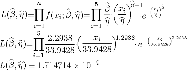
The first step is to calculate the likelihood function for the parameter estimates:

where xi are the original time-to-failure data points. We can now rearrange Eqn. (1) to be:

Since our specified confidence level, δ, is 90%, we can calculate the value of the chi-squared statistic, χ20.9;1 = 2.705543. We then substitute this information into the equation:

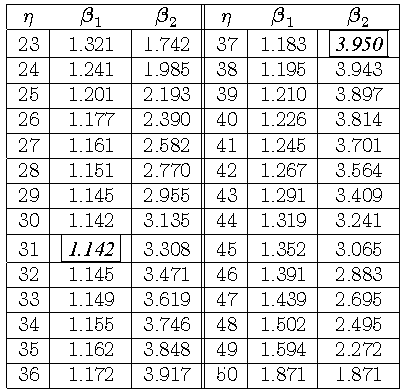
The next step is to find the set of values of β and η that satisfy this equation, or find the values of β and η such that L(β, η) = 4.432926*10-10. The solution is an iterative process that requires setting the value of β and finding the appropriate values of η, and vice versa. The following table gives values of β based on given values of η.

This data set is represented graphically in the following contour plot:

(Note that this plot has been generated with degrees of freedom k = 1, as we are only determining bounds on one parameter. The contour plots generated in Weibull++ are done with degrees of freedom k = 2, for use in comparing both parameters simultaneously.) As can be determined from the table, the lowest calculated value for β is 1.142, while the highest is 3.950. These represent the 2-sided 90% confidence limits on this parameter. Since solutions for the equation do not exist for values of η below 23 or above 50, these can be considered the 90% confidence limits for this parameter. In order to obtain more accurate values for the confidence limits on η, we can perform the same procedure as before, but finding the two values of η that correspond with a given value of β. Using this method, we find that the 90% confidence limits on ηare 22.474 and 49.967, which are close to the initial estimates of 23 and 50.

Note that the points maximum and minimum β points do not necessarily correspond with the maximum and minimum η points. In Part II of this article, we will take a look at how LR bounds can be displayed in the Weibull++ software.