Data Entry Tips for Functions
This topic provides some data entry tips for using spreadsheet functions in ReliaSoft Workbooks and general spreadsheets. If you create the function using the Function Wizard, most of the syntax and formatting issues will be handled automatically. However, you have the option to create or modify function expressions directly in spreadsheet cells.
Note: For DOE design folios, you can disregard any tips related to data source functions(i.e., functions that obtain data or results from a specific data sheet or diagram). For that type of analysis, you can use the DOE Analysis Reports feature to obtain results from a design, multiple linear regression or one-way ANOVA folio, or any of the measurement systems analysis folios.
Case Sensitivity
The functions are not case sensitive.
Entering Text as an Input
When entering text as an input to a function, you must enclose it in quotation marks. This includes situations where you need to specify the data source – DISTR(Weibull!Folio1!Data1) – and situations where you need enter a time or date value in one of the accepted text formats – DAY("22-Aug-2020").
Regional Settings
If your regional settings use a comma as the decimal separator, you must use a semicolon to separate function arguments (e.g., =RELIABILITY("Weibull!Folio1!Data1";A4)).
Referencing a Cell in the Same Sheet
If you want to use another cell in the same sheet, enter the cell reference with a letter to identify the column and a number to identify the row. The cell references can be relative (e.g., B2) or absolute (e.g., $B$2).
- A relative reference points to a cell based on its relative position to the current cell (e.g., B2). When the cell containing the reference is copied, the reference is adjusted to point to a new cell with the same relative offset as the original cell.
- An absolute reference points to a cell at an exact location. Absolute references are designated by placing a dollar sign ($) in front of the row and/or column that is to be absolute. For instance, $B$2 is an absolute reference that points to the cell located in Column B, Row 2 regardless of the position of the cell containing the reference.
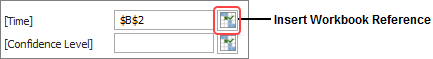
For example, if you want to obtain the probability of failure for the time that has been entered in cell B2, the function could be either =PROBFAIL(B2) or =PROBFAIL($B$2). You can type the cell location directly into the field or click the Function Wizard’s Insert Workbook Reference icon to insert the reference to the cell currently selected in the sheet. If you want to insert an absolute reference, press CTRL while you click the icon.
Another option is to use the Defined Names tool to assign a name to the cell and use the name in all of the function expressions that require that input. (See Defined Names.)
Referencing a Cell in a Different Sheet
To reference a cell in a different sheet from the one in which the formula is entered, use an exclamation mark (!) after the sheet name. For instance, =Sheet1!$B$2 is a reference to the cell located in Column B, Row 2 in Sheet 1. When referencing a cell in a different sheet from the one in which the formula is entered, the reference must be absolute. If the reference is not absolute, the calculations will not be carried out properly.
You can only reference sheets in the same workbook.
Referencing a Cell in a Data Source
Some functions (e.g., DATAENTRY and FMATRIX) require you to reference a particular cell in a data source. This must be defined differently than references to a cell in a spreadsheet. For data source cell references, you must identify first the row and then the column, and use a number rather than a letter to represent the column (e.g., A=1, B=2, C=3 and so on). For example:
- =DATAENTRY(Default1,2,1) returns the value that was entered into cell A2 in the Weibull++ folio that is the data source for this function.
- =FMATRIX(Default1,2,1) returns the value from the second row in the first column of the Fisher variance/covariance matrix that was calculated for that data source.
Creating Composite Functions
It is possible to combine different types of data sources and/or functions to create a composite function. For example, in the following formula, two different data sources are used to return the difference between the reliability at 100 hours calculated from the specific Weibull++ life data folio data sheet called "Weibull!Target!Data1" and the reliability at 100 hours calculated from any given Weibull++ data sheet that is currently first in the list of associated data sources for the workbook or General Spreadsheet.
=(RELIABILITY("Weibull!Target!Data1",100))-(RELIABILITY(Default1,100)
In the next example, nested functions are used to round up the returned reliability result to the nearest two decimals.
=ROUNDUP((RELIABILITY(Default1,1000)),2)
Omitting Optional Inputs in the Middle of a Function
If you do not use an optional input in the middle of the function, the function expression must specifically indicate that the input is being omitted. For example, when using the Weibull++ reliability function (RELIABILITY(Data_Src,Age,[Add Time],[Confidence Level]), if you want to get the confidence bound on the reliability, you must use two commas (,,) to indicate that the [Add Time] input is intentionally blank, before entering the [Confidence Level] in its usual fourth position (e.g., =RELIABILITY(Default1,1000,,0.95)).
Note that this is handled automatically if you use the Function Wizard to build and insert the function expression.
Working with Date Functions
When using one of the spreadsheet date functions (DAY, DAYS360, MONTH, WEEKDAY and YEAR) to enter a date, you can use one of the following accepted text formats:
- Month/Day/Year ("8/22/2019"). For example, =DAY("8/22/2019") returns 22.
- Day-Month-Year ("22-Aug-2019"). For example, =MONTH("22-Aug-2019") returns 8 (because August is the 8th month).
If you do not include the year (e.g., “8/22” or “22-Aug”), the current year is assumed.
Alternatively, you can use the date’s serial number (which is the number of elapsed days since January 1, 1900). For example, =YEAR(43466) returns 2019.
- You can obtain a date's serial number using either of
the following two functions. This may be helpful in cases
where you want to filter, sort or use the date(s)
in calculations.
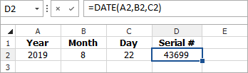
- The DATE function uses the inputs of other cells to obtain the serial number. For example, if you have dates specified in three cells where A2=Year, B2=Month and C2=Day, =DATE(A2,B2,C2) returns the serial number for that date.
- The DATEVALUE function requires you to enter the date in an accepted text format. For example, =DATEVALUE(8/22/2019) returns 43699.
Finally, you can also use the results of other functions within a date function. For example:
- To return the month from today’s current date, use: =MONTH(TODAY())
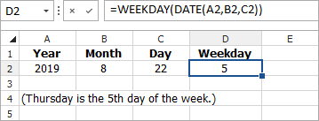
- To return the day of the week for a date that is specified in three separate cells (A2=Year, B2=Month and C2=Day), use: =WEEKDAY(DATE(A2,B2,C2))
Working with Time Functions
When using one of the spreadsheet time functions (HOUR, MINUTE and SECOND) to enter a time, you can use one of the following valid text formats:
- Hour:Minute[:Second] [AM/PM]. For example, =HOUR("4:48:10 PM") returns 16 (the hour using the 24 hour system).
- Month/Day/Year Hour:Minute[:Second] [AM/PM]. For example, =MINUTE("8/22/2019 4:48:10 PM") returns 48.
Alternatively, you can use the hour, minute or second’s serial number (which is the fractional portion of a 24 hour day). For example, =MINUTE(0.70011574) returns 48 (as the specified serial number represents 4:48 PM).
- You can calculate a time's serial number using either
of the following two functions. This may be helpful in cases
where you want to filter, sort or use the time(s)
in calculations
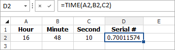
- The TIME function uses the inputs of other cells to obtain the serial number. For example, if you have dates specified in three cells where A2=Hour, B2=Minute and C2=Second, =Time(A2,B2,C2) returns the serial number for that time.
- The TIMEVALUE function requires you to enter the time as text in one of the accepted text formats. For example, =TIMEVALUE(4:48:10 PM) returns 0.70011574.
Finally, you can also use the results of other functions within a time function. For example:
- To generate current values, you can use the NOW function. If the current time is 4:48 PM, then =HOUR(NOW()) returns 16.