QCP Results and Plots for Repairable Systems Analysis
For reliability growth data analysis only.
Weibull++ includes a Quick Calculation Pad (QCP) for computing useful metrics, and multiple plots that allow you to visualize the results of your analyses. The following calculations and plots are available when you are performing repairable systems analysis with the power law or Crow-AMSAA (NHPP) model.
Note: When you analyze data from fielded systems, Weibull++ combines the data to create a single superposition system or cumulative timeline. Any plots generated for the combined data set and subsequent analyses via the Quick Calculation Pad will be based on the resulting system/timeline. See Fielded Data for more information about how the software combines the data for analysis.
QCP Calculations
To open the Quick Calculation Pad (QCP), choose Growth Data > Analysis > Quick Calculation Pad or click the icon on the control panel.
![]()
This section describes the types of calculations you can perform in the QCP for repairable systems analysis. For general information on how to use the QCP, see Quick Calculation Pad (QCP). For information about the metrics and plots available for other types of analyses that you can perform in Weibull++, see QCP Calculations and Plots for Traditional RGA and QCP Calculations and Plots for Crow Extended.
When you are performing repairable systems analysis with a Repairable or Fleet data sheet, the following calculations will be available:
-
Two values can be calculated for either the MTBF or Failure Intensity:
-
The Instantaneous value is the MTBF/FI over a small interval dt that begins at a specified time. For example, an instantaneous MTBF of 5 hours after 100 hours of operation means that, over the next small interval dt that begins at 100 hours, the average time between failures will be 5 hours.
-
The Cumulative value is the MTBF/FI from time = 0 up to a specified end time. For example, a cumulative MTBF of 5 hours from 0 to 100 hours means that the average time between failures was 5 hours over the 100-hour period.
-
-
The Time Given option allows you to calculate the mission duration given any of the following metrics:
-
Cumulative MTBF
-
Instantaneous MTBF
-
Cumulative failure intensity (FI)
-
Instantaneous failure intensity (FI)
-
-
Number of Failures is the cumulative number of failures that are expected to occur by a specified time, based on the fitted model.
-
Expected Fleet Failures is the number of failures that are expected to occur for all systems by a specified time. This option is available only for fielded repairable data and for fielded fleet data.
The following calculations are available only for the Repairable data sheet (which models the number of individual system failures vs. system time, rather than the number of fleet failures vs. fleet time).
- Reliability is the probability that a system that has already operated for a certain amount of time will successfully complete a mission of a certain duration. Enter the amount of time that the system has already operated for in the System Age field, and enter the duration of the mission in the Mission Time field. For example, if the system age = 2 years and mission time = 1 year, the QCP will calculate the reliability for one additional year of operation after the system has already operated for two years (i.e., conditional reliability). To calculate the standard (i.e., non-conditional) reliability, enter 0 for the system age.
- Prob. of Failure is similar to reliability, except that it is the probability that the system will not complete the mission. Thus, it is equal to 1 - Reliability.
- Mission Time is the duration of a mission that a system can complete while still maintaining a certain reliability. Enter the required reliability in the Reliability field, and if you will assume that the system has already operated for a certain time prior to the mission, enter the prior operating time in the System Age field. For example, if system age = 1 year and reliability = 0.9, then the QCP will calculate the longest mission that the system can complete while maintaining a reliability of at least 90%, under the assumption that the system that has already operated for one year.
- Optimum Overhaul is the best time to use between regularly scheduled renewals of the system. By overhauling the system at the right times, you can minimize the total life cycle cost. The optimum overhaul time is calculated using the average Repair Cost and the Overhaul Cost. For example, if it costs $1,000 to repair the system and $3,000 to overhaul it, the QCP can calculate the optimum time to overhaul the system (e.g., every 5 years).
Plots
You can create plots by choosing Growth Data > Analysis > Plot or by clicking the icon on the control panel.
![]()
This section describes the types of plots you can create for repairable systems analysis. The scaling, setup, exporting and confidence bounds settings are similar to the options available for all other reliability growth analysis plot sheets. For more information on these common options, see Plot Utilities.
When you are performing repairable systems analysis with a Repairable or Fleet data sheet, the following plots may be available.
- Cumulative Number of Failures shows the total number of failures versus time. Data points on the plot represent the cumulative number of failures that have been reported by a given time (e.g., the second point marks the time at which the second failure was observed). The Expected Failures line is fitted to the data points and serves as an empirical goodness-of-fit test for the model.
- The [Value] vs. Time plots show how the value increases, decreases or remains constant over time. The points represent the actual failure times in the data set and the plot includes one line for the instantaneous value and one line for the cumulative value.
- System Operation shows the failure times of each system plotted on separate lines. The last line is the timeline for the representative system (i.e., superposition system or cumulative timeline), which is used to evaluate all the failures that occurred during the observation period. To learn more about how the failure times are combined, see Fielded Data.
-
Conditional Reliability/Unreliability is available only when you are using the Repairable data sheet. These plots show the reliability/unreliability versus system age or mission time.
-
If you choose to hold the system age constant, the plots will show the reliability/unreliability for different mission times. For example, assuming that the system has already operated for 100 hours, the plot can show the reliability for the next 10 hours, 20 hours, 30 hours, etc.
-
If you choose to hold mission time constant, the plots will show the reliability/unreliability for different system ages. For example, assuming that the mission will be 100 hours, the plot can show the reliability for a system that has already operated for 10 hours, 20 hours, 30 hours, etc.
To specify which value will be held constant, click the [...] button on the control panel. In the window that appears, select the type of metric that will be held constant, as shown next. Then enter the constant value in the input field.
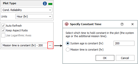
-
- Optimum Overhaul plots are only available when Beta > 1 and only when you are using the Repairable data sheet. These plots show two values; economic life and useful life. Economic life is the overhaul time that minimizes cost (same as the QCP calculation). Useful life takes into account the reliability requirement for the given mission duration. Click Overhaul Settings on the plot control panel to change the parameters.

Tip: Weibull++ includes two additional plot utilities you can use across all types of data: the overlay plot, which allows you to compare different data sets or models; and the side-by-side plot, which allows you to display different plots of a single data set all in a single window for easy comparison.