Appendix B: Additional Information on Load Sharing

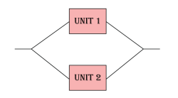
For load sharing systems, one way to model the effect of load on life is to use a life distribution along with a life-stress relationship (as discussed in A Brief Introduction to Life-Stress Relationships) for each component. To illustrate this, consider a system of two units connected reliability-wise in parallel as shown below.

Assume that the units must supply an output of 8 volts and that if both units are operational, each unit is to supply 50% of the total output. If one of the units fails, then the surviving unit supplies 100%. Furthermore, assume that having to supply the entire load has a negative impact on the reliability characteristics of the surviving unit.

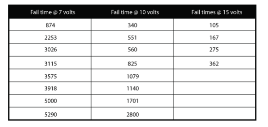
We will create the model starting from raw data. Assume that a total of 20 units were tested to failure at 7, 10 and 15 volts. The test data set is presented in the next table.

For this example, Units 1 and 2 are the same component. Therefore, only one set of data was collected. However, it is possible that the load sharing components in a system may not be the same. If that were the case, data would need to be collected for each component.

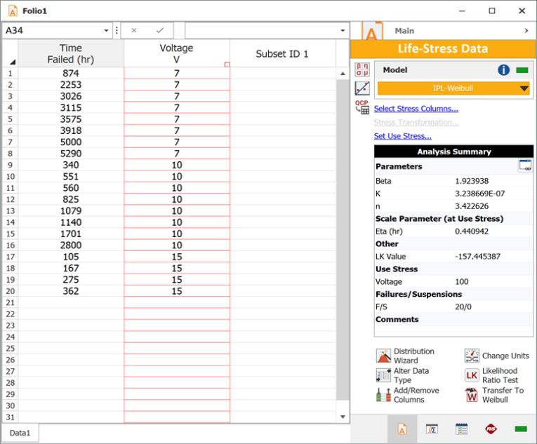
The data set was analyzed using ReliaSoft's ALTA software (as shown in the figure below) with the Inverse Power Law as the underlying life-stress relationship and Weibull as the life distribution.

The estimated model parameters, , and , are shown next.

Or:

.

And for this case:

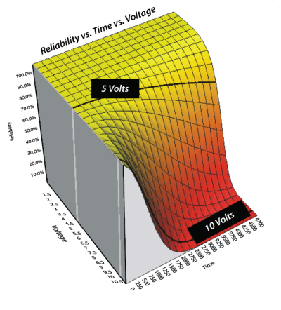
The figure below shows a plot of .

Now that the failure properties have been determined using the test data, the reliability of the system at some time, , can be calculated using the following equation:

where:

and:

• is the total load (or required output).

• and are the portion of the total load that each unit supports when both units are operational. In this case,

• and represent the portions of the load that Unit 1 and Unit 2 must support when both units are operational.

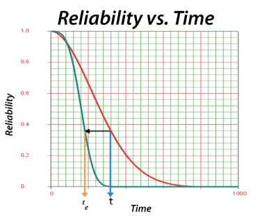
• is the equivalent operating time for Unit 1 if it had been operating at instead of . A graphical representation of the equivalent time is shown in the following figure, where the curve marked by L represents the low stress (load) and the curve marked by H represents the high stress (load).

can be calculated by:

can be calculated the same way, or:

In this example, the reliability equations for Unit 1 and Unit 2 are the same since they are the same type of component and demonstrate the same failure properties. In addition, the total output is divided equally between the two units (when both units are operating), so and will also be the same.

The next step is to determine the reliability of the system after 8,760 hours, . Using

the system reliability is found to be: