Two Level Factorial Designs: Example
The data set used in this example is available in the example database installed with the software (called "Weibull21_DOE_Examples.rsgz21"). To access this database file, choose File > Help, click Open Examples Folder, then browse for the file in the Weibull sub-folder.
The name of the example project is "Factorial - Two Level Full Factorial Design."
One of the initial steps in fabricating integrated circuit (IC) devices is to grow an epitaxial layer on polished silicon wafers. The wafers are mounted on a six-faceted cylinder (two wafers per facet) called a susceptor, which is spun inside a metal bell jar. The jar is injected with chemical vapors through nozzles at the top of the jar and heated. The process continues until the epitaxial layer grows to a desired thickness. The nominal value for thickness is 14.5 µm with specification limits of 14.5 ± 0.5 µm.
The current settings caused variations that exceeded the specification by 1.0 µm. Thus, the experimenters first need to find the factors that affect the process. Then further experiments will be conducted to optimize the process. 96 units are available for testing, and the factors and levels shown next will be used.
|
Factor |
Name |
Low Level |
High Level |
|
A |
Susceptor-Rotation Method |
Continuous |
Oscillating |
|
B |
Nozzle Position |
2 |
6 |
|
C |
Deposition Temperature |
1210 |
1220 |
|
D |
Deposition Time |
Low |
High |
Designing the Experiment
To find the important factors, the experimenters create a two level full factorial design folio, perform the experiment according to the design, and then enter the response values into the folio for analysis. The design matrix and the response data are given in the "Two Level Full Factorial Design" folio. The following steps describe how to create this folio on your own.
- Choose Home > Insert > Standard Design to add a standard design folio to the current project.
![]()
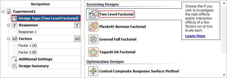
- Click Design Type in the folio's navigation panel, and then select Two Level Factorial in the input panel.
- Rename the response by clicking Response 1 in the navigation panel and entering Thickness in the input panel.
- Specify the number of factors by clicking the Factors heading in the navigation panel and choosing 4 from the Number of Factors drop-down list.
- Define each factor by clicking it in the navigation panel and editing its properties in the input panel. The properties are given in the table above. Note that factors A and D use Qualitative levels; this is specified in the Factor Type drop-down list.
- Rename the folio by clicking the Experiment1 heading in the navigation panel and entering Two Level Factorial Design for the Name in the input panel.
- Click the Additional Settings heading. In the input panel, set the number of Replicates to 6. Note that by leaving Full selected under the Factorial Settings heading, you are indicating that this will be a full factorial design.
- Finally, click the Build icon on the control panel to create a Data tab that allows you to view the test plan and enter response data.
![]()
Analysis and Results
The data set for this example is given in the "Two Level Full Factorial" folio of the example project. After you enter the data from the folio, you can perform the analysis by doing the following:
Note: To minimize the effect of unknown nuisance factors, the run order is randomly generated when you create the design. Therefore, if you followed these steps to create your own folio, the order of runs on the Data tab may be different from that of the folio in the example file. This can lead to different results. To ensure that you get the very same results described next, show the Standard Order column in your folio, then click a cell in that column and choose Sheet > Sheet Actions > Sort > Sort Ascending. This will make the order of runs in your folio the same as that of the example file. Then copy the response data from the example file and paste it into the Data tab of your folio.
- Make sure all main effects and interactions will be considered. To do this, click the Select Terms icon on the control panel.
![]()
In the window that appears, select the All Terms check box. Then click OK.
- Click the Calculate icon.
![]()
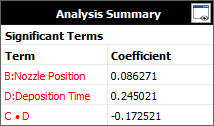
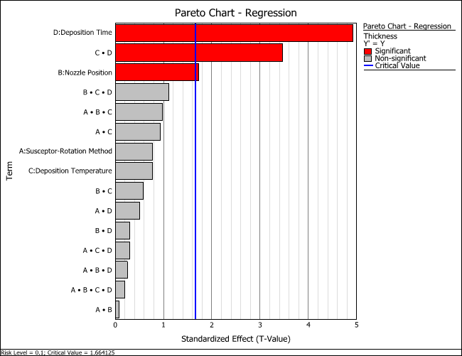
- The results in the Analysis Summary area on the control panel show that the nozzle position and deposition time have significant effects on the thickness, as well as the interaction of terms C and D (i.e., deposition temperature and deposition time).
- To view a plot comparing the standardized effect of each term, click the Plot icon.
![]()
Then choose Pareto Charts - Regression from the Plot Type drop-down list. The following plot appears. The blue line in the plot marks the critical value determined by the risk level specified on the Analysis Settings page of the control panel. If the bar goes past the blue line, then the effect is considered significant.
Optimization
To optimize the response, you should work with a model that only includes the significant terms. The results for the reduced model of the analysis are given in the "Reduced Model" folio of the example project. The following steps describe how to create this folio on your own.
- Right-click the "Two Level Full Factorial Design" folio in the current project explorer. Then choose Duplicate from the shortcut menu.
- Right-click the new, duplicated folio in the current project explorer and choose Rename from the shortcut menu. Change the name to "Reduced Model."
- Open the new folio. Then click the Select Terms icon on the control panel.
![]()
To automatically select only those terms that were found to be significant, click the Select Significant Terms icon. Since the interaction of factors C and D is significant, C must also be included in the model. So select the C:Deposition Temperature check box as well. Then click OK.
- Click the Calculate icon to create a reduced model using the current data.
The factor level combinations that will produce the optimum response value are given in the "Optimal Solution Plot" folio. The following steps describe how to create this folio on your own.
- To find the best settings of the significant factors, click the Design - Optimization icon on the control panel of the "Reduce Mode" folio.
![]()
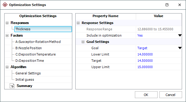
- In the window that appears, use the settings shown next and click OK. According to these settings, the ideal thickness for the epitaxial layer is 14.5 µm, but thicknesses between 14 µm and 15 µm are still acceptable.
- An Optimization folio will appear with an optimal solution plot showing the first solution, displayed next. (The Solutions area on the control panel shows all the solutions that were found, and you can click them to view the plot representing the solution.)
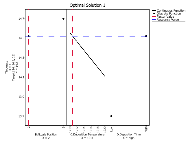
This plot shows one combination of factor settings that will produce the target response value (marked with a horizontal dotted line). Factors B and D are qualitative, so the plot uses dots (i.e., a discrete function) to show what the response level would be given either one of the two factor levels used in the experiment. Factor C is quantitative, so a continuous function is used to calculate the optimal temperature.
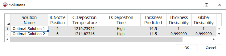
- You can choose Optimization > Solutions > View Solutions or click the icon on the control panel to see all the optimal solutions in numerical format.
![]()
Two optimal solutions for factors B, C and D were found, and they are shown next.
Conclusion
Two optimum solutions were found that give the same predicted thickness. In choosing between these two combinations of factor levels, it is important to identify which is better in terms of variability. To do this, you can perform a variability analysis, where the response is the standard deviation of the observations at each setting. (See Variability Analysis Example.)