Optimal Solution Plot
The optimal solution plot provides a graphical analysis of the factor settings that will produce the user-specified optimum value for one or more responses. This plot is available for all designs with at least two factors.
Creating the Optimal Solution Plot
There are three different ways to create an optimal solution plot:
- On the Home tab, click the Optimization icon in the Insert gallery.
![]()
In the Select Optimization Tool window that appears, select a folio to optimize and then select to create an optimal solution plot.
- You can create an optimal solution plot directly from a calculated design folio by clicking the Optimization icon on the control panel. An optimization folio containing an optimal solution plot for the folio will be added to the DOE folder in the current project explorer. If there is an optimization folio already associated with the design folio, clicking the Optimization icon on the control panel for the design folio will add the optimal solution plot as a sheet within that folio.
- Open an existing optimization folio and add additional optimization tools based on the same design folio by choosing Optimization > Tools > Add Optimization Tool.
Note that each optimization folio can have only one optimization tool of each type.
When you first create an optimal solution plot, you will need to specify the settings that the plot is based on. The Optimization Settings window will appear automatically. The navigation panel on the left of this window lists all of the settings pages.
The pages listed under the Responses heading allow you to select which response(s) you want to optimize, and to specify the optimal settings for each response. The settings on these pages are required in order to create the plot.
Click each response in the navigation panel and use the Include in optimization drop-down list to specify whether the response will be optimized. Note that if a response is missing all data at a given level for a qualitative factor or a block (which is essentially a type of qualitative factor), that level cannot be included in the optimization of the response. Therefore, any optimal solutions found will not use factor levels that do not have data for all selected responses.
The options under the Goal Settings heading allow you to specify whether you want to minimize the response, maximize it or bring it as close as possible to a particular target value. You will then specify a target value for the response, as well as a lower limit and/or an upper limit, depending on the type of goal. These settings affect the desirability rankings of the solutions as follows:
- Target
- Lower Limit: Responses below this value will not be considered desirable at all.
- Target: The closer to this value the response is, the more desirable it is.
- Upper Limit: Responses above this value will not be considered desirable at all.
- Minimize
- Target: Responses below this value will be considered 100% desirable.
- Upper Limit: Responses above this value will not be considered desirable at all.
- Maximize
- Lower Limit: Responses below this value will not be considered desirable at all.
- Target: Responses above this value will be considered 100% desirable.
Note that if a transformation has been applied to any response that you are optimizing, the transformed response values are used in optimization. For this reason, the values that you enter for Lower Limit, Target and/or Upper Limit must also be transformed values. For example, life data responses always have the lognormal transformation applied; therefore, if you are maximizing a life data response, the Lower Limit and Target values should be in terms of Ln(failure time).
If you are including more than one response in the optimization, the Desirability fields will be available. These are used in determining how desirable each optimal solution is.
- Use the Weight field to specify how much the target influences the local desirability of solutions (i.e., how well each solution optimizes that particular response).
- Use the Importance field to specify, on a scale of 0.1 to 10, how much the local desirability of the solution for a given response influences the global desirability of the solution (i.e., how well each solution meets the optimization requirements for all selected responses). This is a way of specifying which response(s) it is most important to optimize (e.g., if one solution does a better job of optimizing Response 1 and another solution does a better job of optimizing Response 2, your inputs in this column will determine which is the more desirable solution).
Inputs for the Weight and Importance are on a scale from 0.1 to 10, where 0.1 is least important and 10 is most important. In other words, if you specify a Weight value of 0.1, response values that are relatively far from the target could still be highly desirable, whereas if you specify a Weight value of 10, only response values extremely close to the target would be highly desirable.
The pages listed under the Factors heading allow you to select which factors will be varied in the optimization, and to specify boundaries or constraints on any quantitative factors to be used in the optimization process, thereby excluding solutions that call for factor settings outside the range(s) you specify. The factor values are expressed in terms of actual or coded values. To change the setting, close the Optimization Settings window and choose Plot > Display > [Value Type].
Click each factor in the navigation panel and use the Treatment in Plot drop-down list to specify whether the factor's value will be varied or held constant during the optimization.
Then use the Lower Limit and Upper Limit fields to specify the bounds for each quantitative factor.
The pages listed under the Algorithm heading allow you to specify how the optimization calculations are performed.
The General Settings page includes the following settings.
- Design Runs specifies the number of runs in the design that will be checked for optimal solutions.
- Random Runs specifies the number of random start points that will be analyzed.
- Epsilon is the convergence criterion that controls how long the software attempts to find optimal solutions. This is for informational purposes and cannot be changed.
- Fractions determines the width of the range from each start point that will be checked for optimal solutions. This is for informational purposes and cannot be changed.
- Use Seed allows the user to specify a start point for the random number generation used in the optimization process, providing repeatability of results.
The Initial Guess page allows you to enter your own estimates of the value for each factor as a starting point for the optimization process. If you do not specify a starting point, random values between the limits specified under the factor settings will be used or, in the case of qualitative factors, every level specified for the qualitative factor is tried for each of the random values of the other factor(s) tried.
To enter a starting point, choose Yes from the Use Initial Guess drop-down list, then enter a value for each factor. For quantitative factors, this will be a numeric value. For qualitative factors and blocks, click inside the field and select the desired option from the drop-down list. If you are supplying initial guesses, you must specify a value for each row.
Note: If optimization does not yield any solutions with a desirability (either global or local) greater than zero, a plot displaying the initial guess value for each factor will be displayed. This not an optimal solution; rather, it is intended to be used as a starting point for manual editing.
The Summary page allows you to review all your optimization settings.
Once you have specified and reviewed the settings, click OK. The software will compute up to five optimal solutions (i.e., the combinations of factor settings that will produce the most desirable response values, based on your specifications in the Optimization Settings window) and will create a plot of the first optimal solution. Other solutions will be displayed in the Solutions area of the control panel; click a solution to view its plot. Note that the order in which the solutions are displayed is random and does not indicate their desirability.
Note:
You can specify new settings and re-compute the optimal solutions
at any time by clicking the Calculate
icon ( ![]() ) to re-open the Optimization Settings
window. You can also change the folio that the optimal solution
plot is based on by clicking the Select
Data Source icon (
) to re-open the Optimization Settings
window. You can also change the folio that the optimal solution
plot is based on by clicking the Select
Data Source icon ( ![]() ).
).
Viewing an Optimal Solution Plot
In the plot of a solution, each response selected for inclusion is presented in a separate row and each factor selected for inclusion is presented in a separate column. In addition, a column can be displayed for blocks. By default, the response value is marked with a blue dashed line and the factor settings that yield that response value are marked with red dashed lines. For example, in the plot shown next, the response is being maximized, with a target value of 4.5 or greater. Three factors are included in the optimization. In this solution, the actual response value of 4.826 is achieved by setting factor A (a qualitative factor) to "copper," factor C (a quantitative factor) to 36.000 and factor E (a qualitative factor) to "new."
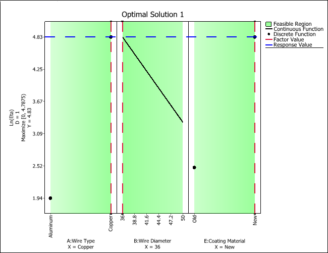
As you can see, possible settings for qualitative factors (and blocks) are displayed as points, while possible settings for quantitative factors are displayed as lines. To change the responses and/or factors that are shown in the plot, click the Select Responses & Factors icon.
![]()
In addition, you can choose to display the feasible region for the factor settings (i.e., the region between the limits specified in the Optimization Settings window) by selecting the Display Feasible Region check box on the control panel. In the plot shown here, the feasible region is indicated by green shading, where reduced desirability is indicated by lighter shading.
Working with Solutions
You can create your own custom solutions by clicking the Create Solution icon ( ![]() ) in the Solutions
area on the control panel. In the window that appears, enter a
name for the solution and specify the factor values to be used
for the solution. Your new solution will be added to the solutions
list.
) in the Solutions
area on the control panel. In the window that appears, enter a
name for the solution and specify the factor values to be used
for the solution. Your new solution will be added to the solutions
list.
Custom solutions can be edited by selecting the solution in
the list and clicking the Edit
Solution icon ( ![]() ) or by dragging the factor lines directly on the plot. Note that
if you edit an optimal solution generated by the software, your
changes will be used to create a new custom solution and the original
solution will remain unchanged. You can also duplicate a solution
by selecting the solution and clicking the Duplicate
Solution icon (
) or by dragging the factor lines directly on the plot. Note that
if you edit an optimal solution generated by the software, your
changes will be used to create a new custom solution and the original
solution will remain unchanged. You can also duplicate a solution
by selecting the solution and clicking the Duplicate
Solution icon ( ![]() ).
).
To remove a solution from the solutions list, select the solution
and click the Delete Solution
icon ( ![]() ). This cannot be undone.
). This cannot be undone.
You can view all of the optimal and custom solutions in a numeric
format by clicking the View Solutions
icon ( ![]() ). The Solutions window shows each solution,
including factor settings, the associated block (if any) and the
predicted response(s) at those settings. The response desirability
columns rate the desirability of each solution from the perspective
of optimizing each response. If more than one solution has been
optimized, the global desirability column rates the overall desirability
of each solution (i.e., how well its relative optimization of
each response meets the requirements specified by the Weight and
Importance settings on the Response Settings tab of the Optimization
Settings window).
). The Solutions window shows each solution,
including factor settings, the associated block (if any) and the
predicted response(s) at those settings. The response desirability
columns rate the desirability of each solution from the perspective
of optimizing each response. If more than one solution has been
optimized, the global desirability column rates the overall desirability
of each solution (i.e., how well its relative optimization of
each response meets the requirements specified by the Weight and
Importance settings on the Response Settings tab of the Optimization
Settings window).
The Transfer Solution to Overlaid
icon ( ![]() ) creates an overlaid contour plot using
the factor values in the currently selected solution.
) creates an overlaid contour plot using
the factor values in the currently selected solution.