The Logistic Distribution
The logistic distribution has been used for growth models, and is used in a certain type of regression known as the logistic regression. It has also applications in modeling life data. The shape of the logistic distribution and the normal distribution are very similar, as discussed in Meeker and Escobar [27]. There are some who argue that the logistic distribution is inappropriate for modeling lifetime data because the left-hand limit of the distribution extends to negative infinity. This could conceivably result in modeling negative times-to-failure. However, provided that the distribution in question has a relatively high mean and a relatively small location parameter, the issue of negative failure times should not present itself as a problem.
Logistic Probability Density Function
The logistic pdf is given by:
where:
Logistic Distribution Functions
Mean, Median and Mode
The logistic mean or MTTF is actually one of the parameters of the distribution, usually denoted as
. Since the logistic distribution is symmetrical,
the median and the mode are always equal to the mean,
Standard Deviation
The standard deviation of the logistic distribution,
, is given by:
The Logistic Reliability Function
The reliability for a mission of time
, starting at age 0, for the logistic distribution is determined by:
or:
The unreliability function is:
where:
The Logistic Conditional Reliability Function
The logistic conditional reliability function is given by:
The Logistic Reliable Life
The logistic reliable life is given by:
The Logistic Failure Rate Function
The logistic failure rate function is given by:
Characteristics of the Logistic Distribution
-
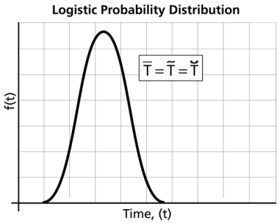
- The logistic distribution has no shape parameter. This means that the logistic pdf has only one shape, the bell shape, and this shape does not change. The shape of the logistic distribution is very similar to that of the normal distribution.
- The mean,
, or the mean life or the
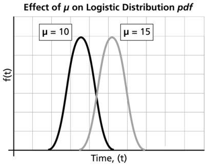
, is also the location parameter of the logistic pdf, as it locates the pdf along the abscissa. It can assume values of
.
- As
decreases, the pdf is shifted to the left.
- As
increases, the pdf is shifted to the right.
-
- As
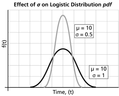
decreases, the pdf gets pushed toward the mean, or it becomes narrower and taller.
- As
increases, the pdf spreads out away from the mean, or it becomes broader and shallower.
- The scale parameter can assume values of
.
- As
-
- The logistic pdf starts at
with an
. As
increases,
also increases, goes through its point of inflection and reaches its maximum value at
. Thereafter,
decreases, goes through its point of inflection and assumes a value of
at
.
- For
the pdf equals 0. The maximum value of the pdf occurs at
and equals
- The point of inflection of the pdf plot is the point where the second derivative of the
pdf equals zero. The inflection point occurs at
or
.
- If the location parameter
decreases, the reliability plot is shifted to the left. If
increases, the reliability plot is shifted to the right.
- If
then
. is the inflection point. If
then
is concave (concave down); if
then
is convex (concave up). For
is convex (concave up), for
is concave (concave down).
- The main difference between the normal distribution and logistic distribution lies in the tails and in the behavior of the failure rate function. The logistic distribution has slightly longer tails compared to the normal distribution. Also, in the upper tail of the logistic distribution, the failure rate function levels out for large
approaching 1/
- If location parameter
decreases, the failure rate plot is shifted to the left. Vice versa if
increases, the failure rate plot is shifted to the right.
always increases. For
for
It is always
- If
increases, then
increases more slowly and smoothly. The segment of time where
increases, too, whereas the region where
is close to 0 or
gets narrower. Conversely, if
decreases, then
increases more quickly and sharply. The segment of time where
decreases, too, whereas the region where
is close to 0 or
gets broader.
- The logistic pdf starts at
Weibull++ Notes on Negative Time Values
One of the disadvantages of using the logistic distribution for reliability calculations is the fact that the logistic distribution starts at negative infinity. This can result in negative values for some of the results. Negative values for time are not accepted in most of the components of Weibull++, nor are they implemented. Certain components of the application reserve negative values for suspensions, or will not return negative results. For example, the Quick Calculation Pad will return a null value (zero) if the result is negative. Only the Free-Form (Probit) data sheet can accept negative values for the random variable (x-axis values).
Logistic Distribution Probability Paper
The form of the Logistic probability paper is based on linearizing the
cdf.
From unreliability equation, can be calculated as a function of the
cdf
as follows:
or using the equation for
Then:
Now let:
and:
which results in the following linear equation:
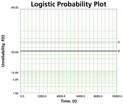
The logistic probability paper resulting from this linearized cdf function is shown next.
Since the logistic distribution is symmetrical, the area under the
pdf curve from to
is 0.5, as is the area from
to
. Consequently, the value of
is said to be the point where
. This means that the estimate of
can be read from the point where the plotted line crosses the 50% unreliability line.
For ,
and
Therefore,
can be found by subtracting
from the time value where the plotted probability line crosses the 73.10% unreliability (26.89% reliability) horizontal line.
Confidence Bounds
In this section, we present the methods used in the application to estimate the different types of confidence bounds for logistically distributed data. The complete derivations were presented in detail (for a general function) in Confidence Bounds.
Bounds on the Parameters
The lower and upper bounds on the location parameter
are estimated from
The lower and upper bounds on the scale parameter
are estimated from:
where is defined by:
If is the confidence level, then
for the two-sided bounds, and
for the one-sided bounds.
The variances and covariances of and
are estimated from the Fisher matrix, as follows:
is the log-likelihood function of the normal distribution, described in
Parameter Estimation and
Appendix D.
Bounds on Reliability
The reliability of the logistic distribution is:
where:
Here ,
,
. Therefore,
also is changing from
to
. Then the bounds on
are estimated from:
where:
or:
The upper and lower bounds on reliability are:
Bounds on Time
The bounds around time for a given logistic percentile (unreliability) are estimated by first solving the reliability equation with respect to time as follows:
where:
or:
The upper and lower bounds are then found by:
General Example
The lifetime of a mechanical valve is known to follow a logistic distribution. 10 units were tested for 28 months and the following months-to-failure data were collected.
| Data Point Index | State F or S | State End Time |
|---|---|---|
| 1 | F | 8 |
| 2 | F | 10 |
| 3 | F | 15 |
| 4 | F | 17 |
| 5 | F | 19 |
| 6 | F | 26 |
| 7 | F | 27 |
| 8 | S | 28 |
| 9 | S | 28 |
| 10 | S | 28 |
- Determine the valve's design life if specifications call for a reliability goal of 0.90.
- The valve is to be used in a pumping device that requires 1 month of continuous operation. What is the probability of the pump failing due to the valve?
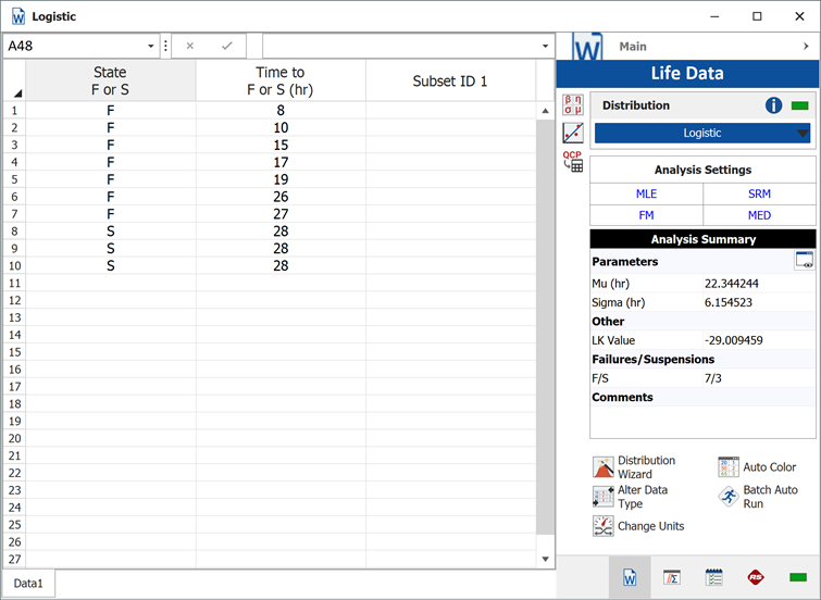
Enter the data set in a Weibull++ standard folio, as follows:
The computed parameters for maximum likelihood are:
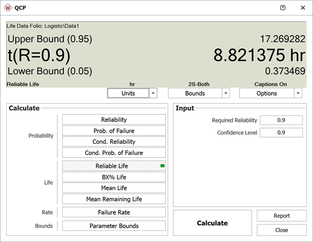
The valve's design life, along with 90% two sided confidence bounds, can be obtained using the QCP as follows:
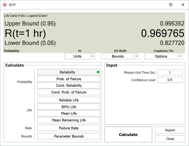
The probability, along with 90% two sided confidence bounds, that the pump fails due to a valve failure during the first month is obtained as follows:




![{\displaystyle {\begin{aligned}{{T}_{R}}=\mu +\sigma [\ln(1-R)-\ln(R)]\end{aligned}}\,\!}](https://en.wikipedia.org/api/rest_v1/media/math/render/svg/717681b00b29d3ead09fa7ce373ed08c5ee24fef)


