The Gamma Distribution
The gamma distribution is a flexible life distribution model that may offer a good fit to some sets of failure data. It is not, however, widely used as a life distribution model for common failure mechanisms. The gamma distribution does arise naturally as the time-to-first-fail distribution for a system with standby exponentially distributed backups, and is also a good fit for the sum of independent exponential random variables. The gamma distribution is sometimes called the Erlang distribution, which is used frequently in queuing theory applications, as discussed in [32].
Gamma Probability Density Function
The pdf of the gamma distribution is given by:
where:
and:
where ,
and
.
Gamma Distribution Functions
Mean, Median and Mode
The gamma mean or MTTF is:
The mode exists if and is given by:
The median is:
Standard Deviation
The standard deviation for the gamma distribution is:
The Gamma Reliability Function
The reliability for a mission of time
for the gamma distribution is:
The Gamma Reliable Life
The gamma reliable life is:
The Gamma Failure Rate Function
The instantaneous gamma failure rate is given by:
Characteristics of the Gamma Distribution
Some of the specific characteristics of the gamma distribution are the following:
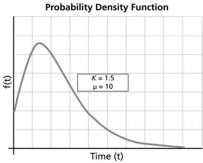
For :
-
- As
,
increases from 0 to the mode value and decreases thereafter.
- If
then pdf has one inflection point at
- If
then pdf has two inflection points for
- For a fixed
, as
increases, the pdf starts to look more like a straight angle.
- As
- As
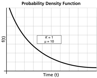
For :
-
- Gamma becomes the exponential distribution.
- As
,
- As
- The pdf decreases monotonically and is convex.
-
.
is constant.
- The mode does not exist.
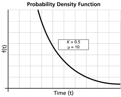
For :
-
- As
,
- As
- As
- The pdf decreases monotonically and is convex.
- As
increases, the pdf gets stretched out to the right and its height decreases, while maintaining its shape.
- As
decreases, the pdf shifts towards the left and its height increases.
- The mode does not exist.
- As
Confidence Bounds
The only method available in Weibull++ for confidence bounds for the gamma distribution is the Fisher matrix, which is described next. The complete derivations were presented in detail (for a general function) in the Confidence Bounds chapter.
Bounds on the Parameters
The lower and upper bounds on the mean,
, are estimated from:
Since the standard deviation, , must be positive,
is treated as normally distributed and the bounds are estimated from:
where is defined by:
If is the confidence level, then
for the two-sided bounds and
for the one-sided bounds.
The variances and covariances of and
are estimated from the Fisher matrix, as follows:
is the log-likelihood function of the gamma distribution, described in
Parameter Estimation and
Appendix D
Bounds on Reliability
The reliability of the gamma distribution is:
where:
The upper and lower bounds on reliability are:
where:
Bounds on Time
The bounds around time for a given gamma percentile (unreliability) are estimated by first solving the reliability equation with respect to time, as follows:
where:
or:
The upper and lower bounds are then found by:
General Example
24 units were reliability tested, and the following life test data were obtained:
| 61 | 50 | 67 | 49 | 53 | 62 |
| 53 | 61 | 43 | 65 | 53 | 56 |
| 62 | 56 | 58 | 55 | 58 | 48 |
| 66 | 44 | 48 | 58 | 43 | 40 |
Fitting the gamma distribution to this data, using maximum likelihood as the analysis method, gives the following parameters:
Using rank regression on the estimated parameters are:
Using rank regression on the estimated parameters are:


