
Appendix D: Confidence Bounds
What Are Confidence Bounds?
One of the most confusing concepts to a novice reliability engineer is estimating the precision of an estimate. This is an important concept in the field of reliability engineering, leading to the use of confidence intervals (or bounds). In this section, we will try to briefly present the concept in relatively simple terms but based on solid common sense.
The Black and White Marbles
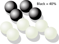
To illustrate, consider the case where there are millions of perfectly mixed black and white marbles in a rather large swimming pool and our job is to estimate the percentage of black marbles. The only way to be absolutely certain about the exact percentage of marbles in the pool is to accurately count every last marble and calculate the percentage. However, this is too time- and resource-intensive to be a viable option, so we need to come up with a way of estimating the percentage of black marbles in the pool. In order to do this, we would take a relatively small sample of marbles from the pool and then count how many black marbles are in the sample.
Taking a Small Sample of Marbles
First, pick out a small sample of marbles and count the black ones. Say you picked out ten marbles and counted four black marbles. Based on this, your estimate would be that 40% of the marbles are black.
If you put the ten marbles back in the pool and repeat this example again, you might get six black marbles, changing your estimate to 60% black marbles. Which of the two is correct? Both estimates are correct! As you repeat this experiment over and over again, you might find out that this estimate is usually between
 and
and
 , and you can assign a percentage to the number of times your estimate falls between these limits. For example, you notice that 90% of the time this estimate is between
 and
and


Taking a Larger Sample of Marbles
If you now repeat the experiment and pick out 1,000 marbles, you might get results for the number of black marbles such as 545, 570, 530, etc., for each trial. The range of the estimates in this case will be much narrower than before. For example, you observe that 90% of the time, the number of black marbles will now be from
 to
to
 , where
 and
and
 , thus giving you a more narrow estimate interval. The same principle is true for confidence intervals; the larger the sample size, the more narrow the confidence intervals.


Back to Reliability
We will now look at how this phenomenon relates to reliability. Overall, the reliability engineer's task is to determine the probability of failure, or reliability, of the population of units in question. However, one will never know the exact reliability value of the population unless one is able to obtain and analyze the failure data for every single unit in the population. Since this usually is not a realistic situation, the task then is to estimate the reliability based on a sample, much like estimating the number of black marbles in the pool. If we perform ten different reliability tests for our units, and analyze the results, we will obtain slightly different parameters for the distribution each time, and thus slightly different reliability results. However, by employing confidence bounds, we obtain a range within which these reliability values are likely to occur a certain percentage of the time. This helps us gauge the utility of the data and the accuracy of the resulting estimates. Plus, it is always useful to remember that each parameter is an estimate of the true parameter, one that is unknown to us. This range of plausible values is called a confidence interval.
One-Sided and Two-Sided Confidence Bounds
Confidence bounds are generally described as being one-sided or two-sided.
Two-Sided Bounds
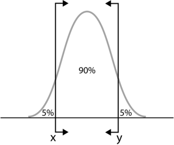
When we use two-sided confidence bounds (or intervals), we are looking at a closed interval where a certain percentage of the population is likely to lie. That is, we determine the values, or bounds, between which lies a specified percentage of the population. For example, when dealing with 90% two-sided confidence bounds of
 , we are saying that 90% of the population lies between
 and
and
 with 5% less than
 and 5% greater than
 .
.


One-Sided Bounds
One-sided confidence bounds are essentially an open-ended version of two-sided bounds. A one-sided bound defines the point where a certain percentage of the population is either higher or lower than the defined point. This means that there are two types of one-sided bounds: upper and lower. An upper one-sided bound defines a point that a certain percentage of the population is less than. Conversely, a lower one-sided bound defines a point that a specified percentage of the population is greater than.
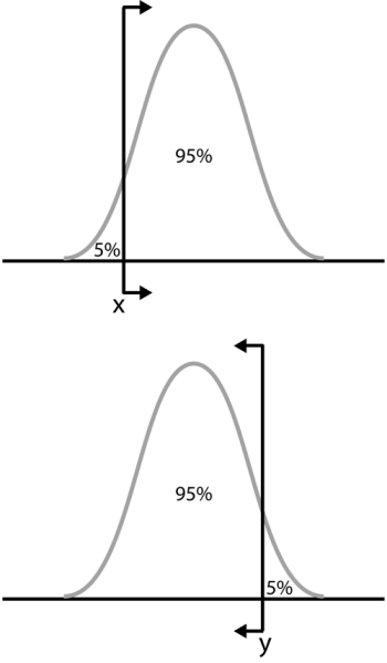
For example, if  is a 95% upper one-sided bound, this would imply that 95% of the population is less than
 . If
. If
 is a 95% lower one-sided bound, this would indicate that 95% of the population is greater than
 . Care must be taken to differentiate between one- and two-sided confidence bounds, as these bounds can take on identical values at different percentage levels. For example, in the figures above, we see bounds on a hypothetical distribution. Assuming that this is the same distribution in all of the figures, we see that
 marks the spot below which 5% of the distribution's population lies. Similarly,
 represents the point above which 5% of the population lies. Therefore,
 and
and
 represent the 90% two-sided bounds, since 90% of the population lies between the two points. However,
 also represents the lower one-sided 95% confidence bound, since 95% of the population lies above that point; and
 represents the upper one-sided 95% confidence bound, since 95% of the population is below
 . It is important to be sure of the type of bounds you are dealing with, particularly as both one-sided bounds can be displayed simultaneously in Weibull++. In Weibull++, we use upper to represent the higher limit and lower to represent the lower limit, regardless of their position, but based on the value of the results. So if obtaining the confidence bounds on the reliability, we would identify the lower value of reliability as the lower limit and the higher value of reliability as the higher limit. If obtaining the confidence bounds on probability of failure we will again identify the lower numeric value for the probability of failure as the lower limit and the higher value as the higher limit.
Fisher Matrix Confidence Bounds
This section presents an overview of the theory on obtaining approximate confidence bounds on suspended (multiple censored) data. The methodology used is the so-called Fisher matrix bounds (FM), described in Nelson
[30] and Lloyd and Lipow
[24]. These bounds are employed in most other commercial statistical applications. In general, these bounds tend to be more optimistic than the non-parametric rank based bounds. This may be a concern, particularly when dealing with small sample sizes. Some statisticians feel that the Fisher matrix bounds are too optimistic when dealing with small sample sizes and prefer to use other techniques for calculating confidence bounds, such as the likelihood ratio bounds.
Approximate Estimates of the Mean and Variance of a Function
In utilizing FM bounds for functions, one must first determine the mean and variance of the function in question (i.e., reliability function, failure rate function, etc.). An example of the methodology and assumptions for an arbitrary function
 is presented next.

Single Parameter Case
For simplicity, consider a one-parameter distribution represented by a general function
 which is a function of one parameter estimator, say
 For example, the mean of the exponential distribution is a function of the parameter
 . Then, in general, the expected value of
 can be found by:


where  is some function of
 , such as the reliability function, and
 is the population parameter where
 as
as
 . The term
 is a function of
 , the sample size, and tends to zero, as fast as
 as
as
 For example, in the case of
 and
and
 , then
 where
where
 . Thus as
 ,
,
 where
where
 and
and
 are the mean and standard deviation, respectively. Using the same one-parameter distribution, the variance of the function
 can then be estimated by:


Two-Parameter Case
Consider a Weibull distribution with two parameters
 and
and
 . For a given value of
 ,
,
 . Repeating the previous method for the case of a two-parameter distribution, it is generally true that for a function
 , which is a function of two parameter estimators, say
 , that:


and:


Note that the derivatives of the above equation are evaluated at
 and
and
 where E
 and E
and E


Parameter Variance and Covariance Determination
The determination of the variance and covariance of the parameters is accomplished via the use of the Fisher information matrix. For a two-parameter distribution, and using maximum likelihood estimates (MLE), the log-likelihood function for censored data is given by:

![{\displaystyle {\begin{aligned}\ln[L]=&\Lambda ={\underset {i=1}{\overset {R}{\mathop {\sum } }}}\,\ln[f({{T}_{i}};{{\theta }_{1}},{{\theta }_{2}})]\\&{\text{ }}+{\underset {j=1}{\overset {M}{\mathop {\sum } }}}\,\ln[1-F({{S}_{j}};{{\theta }_{1}},{{\theta }_{2}})]\\&{\text{ }}+{\underset {l=1}{\overset {P}{\mathop {\sum } }}}\,\ln \left\{F({{I}_{{l}_{U}}};{{\theta }_{1}},{{\theta }_{2}})-F({{I}_{{l}_{L}}};{{\theta }_{1}},{{\theta }_{2}})\right\}\end{aligned}}\,\!}](https://en.wikipedia.org/api/rest_v1/media/math/render/svg/e061e3e5629095590ce223090cdd08f7e51b0bfc)
In the equation above, the first summation is for complete data, the second summation is for right censored data and the third summation is for interval or left censored data.
Then the Fisher information matrix is given by:

![{\displaystyle {{F}_{0}}=\left[{\begin{matrix}{{E}_{0}}{{\left[-{\tfrac {{{\partial }^{2}}\Lambda }{\partial \theta _{1}^{2}}}\right]}_{0}}&{}&{{E}_{0}}{{\left[-{\tfrac {{{\partial }^{2}}\Lambda }{\partial {{\theta }_{1}}\partial {{\theta }_{2}}}}\right]}_{0}}\\{}&{}&{}\\{{E}_{0}}{{\left[-{\tfrac {{{\partial }^{2}}\Lambda }{\partial {{\theta }_{2}}\partial {{\theta }_{1}}}}\right]}_{0}}&{}&{{E}_{0}}{{\left[-{\tfrac {{{\partial }^{2}}\Lambda }{\partial \theta _{2}^{2}}}\right]}_{0}}\\\end{matrix}}\right]\,\!}](https://en.wikipedia.org/api/rest_v1/media/math/render/svg/358b85d7a281b712e73fe617533cad13b5a5d19e)
The subscript 0 indicates that the quantity is evaluated at
 and
and
 the true values of the parameters.


So for a sample of  units where
 units have failed,
 have been suspended, and
 have failed within a time interval, and
 one could obtain the sample local information matrix by:


![{\displaystyle F={{\left[{\begin{matrix}-{\tfrac {{{\partial }^{2}}\Lambda }{\partial \theta _{1}^{2}}}&{}&-{\tfrac {{{\partial }^{2}}\Lambda }{\partial {{\theta }_{1}}\partial {{\theta }_{2}}}}\\{}&{}&{}\\-{\tfrac {{{\partial }^{2}}\Lambda }{\partial {{\theta }_{2}}\partial {{\theta }_{1}}}}&{}&-{\tfrac {{{\partial }^{2}}\Lambda }{\partial \theta _{2}^{2}}}\\\end{matrix}}\right]}^{}}\,\!}](https://en.wikipedia.org/api/rest_v1/media/math/render/svg/41fdf0358810cb47b88015993dd59e746d3e0062)
Substituting the values of the estimated parameters, in this case
 and
and
 , and then inverting the matrix, one can then obtain the local estimate of the covariance matrix or:


![{\displaystyle \left[{\begin{matrix}{\widehat {Var}}\left({{\widehat {\theta }}_{1}}\right)&{}&{\widehat {Cov}}\left({{\widehat {\theta }}_{1}},{{\widehat {\theta }}_{2}}\right)\\{}&{}&{}\\{\widehat {Cov}}\left({{\widehat {\theta }}_{1}},{{\widehat {\theta }}_{2}}\right)&{}&{\widehat {Var}}\left({{\widehat {\theta }}_{2}}\right)\\\end{matrix}}\right]={{\left[{\begin{matrix}-{\tfrac {{{\partial }^{2}}\Lambda }{\partial \theta _{1}^{2}}}&{}&-{\tfrac {{{\partial }^{2}}\Lambda }{\partial {{\theta }_{1}}\partial {{\theta }_{2}}}}\\{}&{}&{}\\-{\tfrac {{{\partial }^{2}}\Lambda }{\partial {{\theta }_{2}}\partial {{\theta }_{1}}}}&{}&-{\tfrac {{{\partial }^{2}}\Lambda }{\partial \theta _{2}^{2}}}\\\end{matrix}}\right]}^{-1}}\,\!}](https://en.wikipedia.org/api/rest_v1/media/math/render/svg/e14761b7fe132c7c84e5e957fcc2cc8f7e3f7cb3)
Then the variance of a function ( ) can be estimated using equation for the variance. Values for the variance and covariance of the parameters are obtained from Fisher Matrix equation. Once they have been obtained, the approximate confidence bounds on the function are given as:


which is the estimated value plus or minus a certain number of standard deviations. We address finding
 next.
next.

Approximate Confidence Intervals on the Parameters
In general, MLE estimates of the parameters are asymptotically normal, meaning that for large sample sizes, a distribution of parameter estimates from the same population would be very close to the normal distribution. Thus if
 is the MLE estimator for
 , in the case of a single parameter distribution estimated from a large sample of
 units, then:


follows an approximating normal distribution. That is


for large  . We now place confidence bounds on
 at some confidence level
 , bounded by the two end points
 and
and
 where:


From the above equation:


where  is defined by:


Now by simplifying the equation for the confidence level, one can obtain the approximate two-sided confidence bounds on the parameter
 at a confidence level
 or:
or:


The upper one-sided bounds are given by:


while the lower one-sided bounds are given by:


If  must be positive, then
 is treated as normally distributed. The two-sided approximate confidence bounds on the parameter
 , at confidence level
 , then become:


The one-sided approximate confidence bounds on the parameter
 , at confidence level
 can be found from:


The same procedure can be extended for the case of a two or more parameter distribution. Lloyd and Lipow [24] further elaborate on this procedure.
Confidence Bounds on Time (Type 1)
Type 1 confidence bounds are confidence bounds around time for a given reliability. For example, when using the one-parameter exponential distribution, the corresponding time for a given exponential percentile (i.e., y-ordinate or unreliability,
 is determined by solving the unreliability function for the time,
 , or:
, or:


Bounds on time (Type 1) return the confidence bounds around this time value by determining the confidence intervals around
 and substituting these values into the above equation. The bounds on
 are determined using the method for the bounds on parameters, with its variance obtained from the Fisher Matrix. Note that the procedure is slightly more complicated for distributions with more than one parameter.

Confidence Bounds on Reliability (Type 2)
Type 2 confidence bounds are confidence bounds around reliability. For example, when using the two-parameter exponential distribution, the reliability function is:


Reliability bounds (Type 2) return the confidence bounds by determining the confidence intervals around
 and substituting these values into the above equation. The bounds on
 are determined using the method for the bounds on parameters, with its variance obtained from the Fisher Matrix. Once again, the procedure is more complicated for distributions with more than one parameter.
Beta Binomial Confidence Bounds
Another less mathematically intensive method of calculating confidence bounds involves a procedure similar to that used in calculating median ranks (see
Parameter Estimation). This is a non-parametric approach to confidence interval calculations that involves the use of rank tables and is commonly known as beta-binomial bounds (BB). By non-parametric, we mean that no underlying distribution is assumed. (Parametric implies that an underlying distribution, with parameters, is assumed.) In other words, this method can be used for any distribution, without having to make adjustments in the underlying equations based on the assumed distribution. Recall from the discussion on the median ranks that we used the binomial equation to compute the ranks at the 50% confidence level (or median ranks) by solving the cumulative binomial distribution for
 (rank for the
 failure):


where  is the sample size and
 is the order number.

The median rank was obtained by solving the following equation for
 :
:


The same methodology can then be repeated by changing
 for 0.50 (50%) to our desired confidence level. For
 one would formulate the equation as


Keep in mind that one must be careful to select the appropriate values for
 based on the type of confidence bounds desired. For example, if two-sided 80% confidence bounds are to be calculated, one must solve the equation twice (once with
 and once with
 ) in order to place the bounds around 80% of the population.


Using this methodology, the appropriate ranks are obtained and plotted based on the desired confidence level. These points are then joined by a smooth curve to obtain the corresponding confidence bound.
In Weibull++, this non-parametric methodology is used only when plotting bounds on the mixed Weibull distribution. Full details on this methodology can be found in Kececioglu [20]. These binomial equations can again be transformed using the beta and F distributions, thus the name beta binomial confidence bounds.
Likelihood Ratio Confidence Bounds
Another method for calculating confidence bounds is the likelihood ratio bounds (LRB) method. Conceptually, this method is a great deal simpler than that of the Fisher matrix, although that does not mean that the results are of any less value. In fact, the LRB method is often preferred over the FM method in situations where there are smaller sample sizes.
Likelihood ratio confidence bounds are based on the following likelihood ratio equation:


where:
-
 is the likelihood function for the unknown parameter vector

 is the likelihood function calculated at the estimated vector

 is the chi-squared statistic with probability
 and
and
 degrees of freedom, where
 is the number of quantities jointly estimated


If  is the confidence level, then
 for two-sided bounds and
 for one-sided. Recall from the
Brief Statistical Background chapter that if
for one-sided. Recall from the
Brief Statistical Background chapter that if
 is a continuous random variable with
pdf:
is a continuous random variable with
pdf:


where  are
are
 unknown constant parameters that need to be estimated, one can conduct an experiment and obtain
 independent observations,
 , which correspond in the case of life data analysis to failure times. The likelihood function is given by:


The maximum likelihood estimators (MLE) of
 are
are
 are obtained by maximizing
 These are represented by the
 term in the denominator of the ratio in the likelihood ratio equation. Since the values of the data points are known, and the values of the parameter estimates
 have been calculated using MLE methods, the only unknown term in the likelihood ratio equation is the
 term in the numerator of the ratio. It remains to find the values of the unknown parameter vector
 that satisfy the likelihood ratio equation. For distributions that have two parameters, the values of these two parameters can be varied in order to satisfy the likelihood ratio equation. The values of the parameters that satisfy this equation will change based on the desired confidence level
 but at a given value of
 there is only a certain region of values for
 and
and
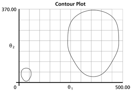
 for which the likelihood ratio equation holds true. This region can be represented graphically as a contour plot, an example of which is given in the following graphic.


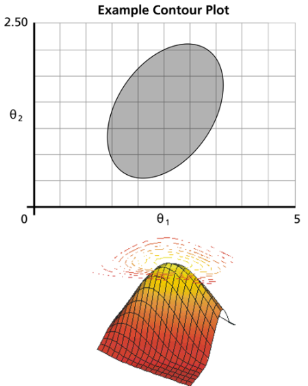
The region of the contour plot essentially represents a cross-section of the likelihood function surface that satisfies the conditions of the likelihood ratio equation.
Note on Contour Plots in Weibull++
Contour plots can be used for comparing data sets. Consider two data sets, one for an&.html#160;old product design and another for a new design. The engineer would like to determine if the two designs are significantly different and at what confidence. By plotting the contour plots of each data set in an overlay plot (the same distribution must be fitted to each data set), one can determine the confidence at which the two sets are significantly different. If, for example, there is no overlap (i.e., the two plots do not intersect) between the two 90% contours, then the two data sets are significantly different with a 90% confidence. If the two 95% contours overlap, then the two designs are NOT significantly different at the 95% confidence level. An example of non-intersecting contours is shown next. For details on comparing data sets, see Comparing Life Data Sets.
Confidence Bounds on the Parameters
The bounds on the parameters are calculated by finding the extreme values of the contour plot on each axis for a given confidence level. Since each axis represents the possible values of a given parameter, the boundaries of the contour plot represent the extreme values of the parameters that satisfy the following:


This equation can be rewritten as:


The task now is to find the values of the parameters
 and
and
 so that the equality in the likelihood ratio equation shown above is satisfied. Unfortunately, there is no closed-form solution; therefore, these values must be arrived at numerically. One way to do this is to hold one parameter constant and iterate on the other until an acceptable solution is reached. This can prove to be rather tricky, since there will be two solutions for one parameter if the other is held constant. In situations such as these, it is best to begin the iterative calculations with values close to those of the MLE values, so as to ensure that one is not attempting to perform calculations outside of the region of the contour plot where no solution exists.
Example 1:Likelihood Ratio Bounds on Parameters
Five units were put on a reliability test and experienced failures at 10, 20, 30, 40 and 50 hours. Assuming a Weibull distribution, the MLE parameter estimates are calculated to be
 and
and
 Calculate the 90% two-sided confidence bounds on these parameters using the likelihood ratio method.


Solution
The first step is to calculate the likelihood function for the parameter estimates:


where  are the original time-to-failure data points. We can now rearrange the likelihood ratio equation to the form:


Since our specified confidence level,
 , is 90%, we can calculate the value of the chi-squared statistic,
 We then substitute this information into the equation:


The next step is to find the set of values of
 and
and
 that satisfy this equation, or find the values of
 and
and
 such that


The solution is an iterative process that requires setting the value of
 and finding the appropriate values of
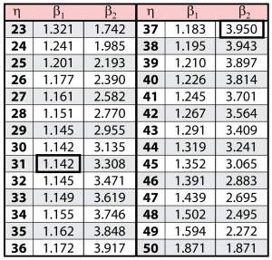
 , and vice versa. The following table gives values of
 based on given values of
 .
.
These data are represented graphically in the following contour plot:
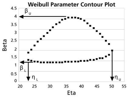
(Note that this plot is generated with degrees of freedom
 , as we are only determining bounds on one parameter. The contour plots generated in Weibull++ are done with degrees of freedom
 , for use in comparing both parameters simultaneously.) As can be determined from the table, the lowest calculated value for
 is 1.142, while the highest is 3.950. These represent the two-sided 90% confidence limits on this parameter. Since solutions for the equation do not exist for values of
 below 23 or above 50, these can be considered the 90% confidence limits for this parameter. In order to obtain more accurate values for the confidence limits on
 , we can perform the same procedure as before, but finding the two values of
 that correspond with a given value of
 Using this method, we find that the 90% confidence limits on
 are 22.474 and 49.967, which are close to the initial estimates of 23 and 50.


Note that the points where  are maximized and minimized do not necessarily correspond with the points where
 are maximized and minimized. This is due to the fact that the contour plot is not symmetrical, so that the parameters will have their extremes at different points.
Confidence Bounds on Time (Type 1)
The manner in which the bounds on the time estimate for a given reliability are calculated is much the same as the manner in which the bounds on the parameters are calculated. The difference lies in the form of the likelihood functions that comprise the likelihood ratio. In the preceding section, we used the standard form of the likelihood function, which was in terms of the parameters
 and
and
 . In order to calculate the bounds on a time estimate, the likelihood function needs to be rewritten in terms of one parameter and time, so that the maximum and minimum values of the time can be observed as the parameter is varied. This process is best illustrated with an example.
Example 2:Likelihood Ratio Bounds on Time (Type I)
For the data given in Example 1, determine the 90% two-sided confidence bounds on the time estimate for a reliability of 50%. The ML estimate for the time at which
 is 28.930.

Solution
In this example, we are trying to determine the 90% two-sided confidence bounds on the time estimate of 28.930. As was mentioned, we need to rewrite the likelihood ratio equation so that it is in terms of
 and
and
 This is accomplished by using a form of the Weibull reliability equation,
 This can be rearranged in terms of
 , with
 being considered a known variable or:


This can then be substituted into the
 term in the likelihood ratio equation to form a likelihood equation in terms of
 and
and
 or:
or:


![{\displaystyle ={\underset {i=1}{\overset {5}{\mathop {\prod } }}}\,{\frac {\beta }{\left({\tfrac {t}{{(-{\text{ln}}(R))}^{\tfrac {1}{\beta }}}}\right)}}\cdot {{\left({\frac {{x}_{i}}{\left({\tfrac {t}{{(-{\text{ln}}(R))}^{\tfrac {1}{\beta }}}}\right)}}\right)}^{\beta -1}}\cdot {\text{exp}}\left[-{{\left({\frac {{x}_{i}}{\left({\tfrac {t}{{(-{\text{ln}}(R))}^{\tfrac {1}{\beta }}}}\right)}}\right)}^{\beta }}\right]\,\!}](https://en.wikipedia.org/api/rest_v1/media/math/render/svg/586683520f3b8150e35488e1fde8ad2fd3c7c2fc)
where  are the original time-to-failure data points. We can now rearrange the likelihood ratio equation to the form:


Since our specified confidence level,
 , is 90%, we can calculate the value of the chi-squared statistic,
 We can now substitute this information into the equation:


Note that the likelihood value for  is the same as it was for Example 1. This is because we are dealing with the same data and parameter estimates or, in other words, the maximum value of the likelihood function did not change. It now remains to find the values of
 and
and
 which satisfy this equation. This is an iterative process that requires setting the value of
 and finding the appropriate values of
 . The following table gives the values of
 based on given values of
 .
.

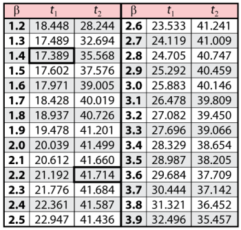
These points are represented graphically in the following contour plot:
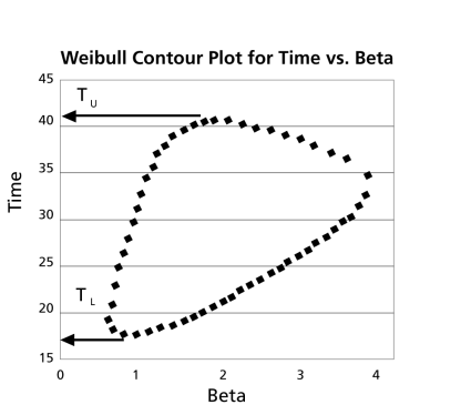
As can be determined from the table, the lowest calculated value for
 is 17.389, while the highest is 41.714. These represent the 90% two-sided confidence limits on the time at which reliability is equal to 50%.
Confidence Bounds on Reliability (Type 2)
The likelihood ratio bounds on a reliability estimate for a given time value are calculated in the same manner as were the bounds on time. The only difference is that the likelihood function must now be considered in terms of
 and
and
 . The likelihood function is once again altered in the same way as before, only now
 is considered to be a parameter instead of
 , since the value of
 must be specified in advance. Once again, this process is best illustrated with an example.
Example 3:Likelihood Ratio Bounds on Reliability (Type 2)
For the data given in Example 1, determine the 90% two-sided confidence bounds on the reliability estimate for
 . The ML estimate for the reliability at
 is 14.816%.

Solution
In this example, we are trying to determine the 90% two-sided confidence bounds on the reliability estimate of 14.816%. As was mentioned, we need to rewrite the likelihood ratio equation so that it is in terms of
 and
and
 This is again accomplished by substituting the Weibull reliability equation into the
 term in the likelihood ratio equation to form a likelihood equation in terms of
 and
and
 :
:


where  are the original time-to-failure data points. We can now rearrange the likelihood ratio equation to the form:


Since our specified confidence level,
 , is 90%, we can calculate the value of the chi-squared statistic,
 We can now substitute this information into the equation:


It now remains to find the values of
 and
and
 that satisfy this equation. This is an iterative process that requires setting the value of
 and finding the appropriate values of
 . The following table gives the values of
 based on given values of
 .
.
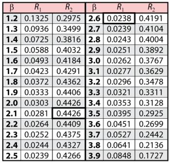
These points are represented graphically in the following contour plot:
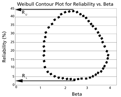
As can be determined from the table, the lowest calculated value for
 is 2.38%, while the highest is 44.26%. These represent the 90% two-sided confidence limits on the reliability at
 .
.
Bayesian Confidence Bounds
A fourth method of estimating confidence bounds is based on the Bayes theorem. This type of confidence bounds relies on a different school of thought in statistical analysis, where prior information is combined with sample data in order to make inferences on model parameters and their functions. An introduction to Bayesian methods is given in the Parameter Estimation chapter. Bayesian confidence bounds are derived from Bayes's rule, which states that:


where:
-
 ) is the
posterior pdf of
) is the
posterior pdf of 
 is the parameter vector of the chosen distribution (i.e., Weibull, lognormal, etc.)
 is the likelihood function
 is the
prior pdf of the parameter vector
is the
prior pdf of the parameter vector

 is the range of
 .
.


In other words, the prior knowledge is provided in the form of the prior
pdf of the parameters, which in turn is combined with the sample data in order to obtain the posterior
pdf. Different forms of prior information exist, such as past data, expert opinion or non-informative (refer to
Parameter Estimation). It can be seen from the above Bayes's rule formula that we are now dealing with distributions of parameters rather than single value parameters. For example, consider a one-parameter distribution with a positive parameter
 . Given a set of sample data, and a prior distribution for

 the above Bayes's rule formula can be written as:


In other words, we now have the distribution of
 and we can now make statistical inferences on this parameter, such as calculating probabilities. Specifically, the probability that
 is less than or equal to a value

 can be obtained by integrating the posterior probability density function (pdf), or:


The above equation is the posterior cdf, which essentially calculates a confidence bound on the parameter, where
 is the confidence level and
 is the confidence bound. Substituting the posterior
pdf into the above posterior cdf yields:
is the confidence bound. Substituting the posterior
pdf into the above posterior cdf yields:


The only question at this point is, what do we use as a prior distribution of
 ? For the confidence bounds calculation application, non-informative prior distributions are utilized. Non-informative prior distributions are distributions that have no population basis and play a minimal role in the posterior distribution. The idea behind the use of non-informative prior distributions is to make inferences that are not affected by external information, or when external information is not available. In the general case of calculating confidence bounds using Bayesian methods, the method should be independent of external information and it should only rely on the current data. Therefore, non-informative priors are used. Specifically, the uniform distribution is used as a prior distribution for the different parameters of the selected fitted distribution. For example, if the Weibull distribution is fitted to the data, the prior distributions for beta and eta are assumed to be uniform. The above equation can be generalized for any distribution having a vector of parameters
 yielding the general equation for calculating Bayesian confidence bounds:


where:
-
 is the confidence level
 is the parameter vector
 is the likelihood function
 is the prior
pdf of the parameter vector
is the prior
pdf of the parameter vector

 is the range of

 is the range in which
 changes from
 till
till
 's maximum value, or from
 's minimum value till

 is a function such that if
 is given, then the bounds are calculated for
 . If
. If
 is given, then the bounds are calculated for
 .
.


If  is given, then from the above equation and
 and for a given
 , the bounds on
 are calculated. If
 is given, then from the above equation and
 and for a given
 the bounds on
 are calculated.


Confidence Bounds on Time (Type 1)
For a given failure time distribution and a given reliability
 ,
,
 is a function of
 and the distribution parameters. To illustrate the procedure for obtaining confidence bounds, the two-parameter Weibull distribution is used as an example. The bounds in other types of distributions can be obtained in similar fashion. For the two-parameter Weibull distribution:


For a given reliability, the Bayesian one-sided upper bound estimate for
 is:
is:


where  is the posterior distribution of Time
 Using the above equation, we have the following:


The above equation can be rewritten in terms of
 as:
as:


Applying the Bayes's rule by assuming that the priors of
 and
and
 are independent, we then obtain the following relationship:


The above equation can be solved for
 , where:

-
 is the confidence level,
 is the prior
pdf of the parameter
is the prior
pdf of the parameter  . For non-informative prior distribution,

 is the prior
pdf of the parameter
is the prior
pdf of the parameter  For non-informative prior distribution,

 is the likelihood function.


The same method can be used to get the one-sided lower bound of
 from:
from:


The above equation can be solved to get
 .
.

The Bayesian two-sided bounds estimate for
 is:
is:


which is equivalent to:


and:


Using the same method for the one-sided bounds,
 and
and
 can be solved.
Confidence Bounds on Reliability (Type 2)
For a given failure time distribution and a given time
 ,
,
 is a function of
 and the distribution parameters. To illustrate the procedure for obtaining confidence bounds, the two-parameter Weibull distribution is used as an example. The bounds in other types of distributions can be obtained in similar fashion. For example, for two parameter Weibull distribution:


The Bayesian one-sided upper bound estimate for
 is:
is:


Similar to the bounds on Time, the following is obtained:


The above equation can be solved to get
 .
.

The Bayesian one-sided lower bound estimate for R(T) is:


Using the posterior distribution, the following is obtained:


The above equation can be solved to get
 .
.

The Bayesian two-sided bounds estimate for
 is:
is:


which is equivalent to:


and


Using the same method for one-sided bounds,
 and
and
 can be solved.
Simulation Based Bounds
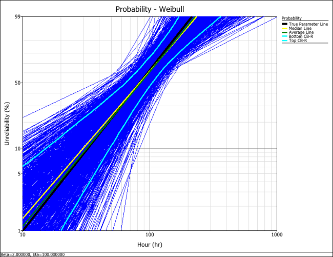
The SimuMatic tool in Weibull++ can be used to perform a large number of reliability analyses on data sets that have been created using Monte Carlo simulation. This utility can assist the analyst to a) better understand life data analysis concepts, b) experiment with the influences of sample sizes and censoring schemes on analysis methods, c) construct simulation-based confidence intervals, d) better understand the concepts behind confidence intervals and e) design reliability tests. This section describes how to use simulation for estimating confidence bounds.
SimuMatic generates confidence bounds and assists in visualizing and understanding them. In addition, it allows one to determine the adequacy of certain parameter estimation methods (such as rank regression on X, rank regression on Y and maximum likelihood estimation) and to visualize the effects of different data censoring schemes on the confidence bounds.
Example:Comparing Parameter Estimation Methods Using Simulation Based Bounds
The purpose of this example is to determine the best parameter estimation method for a sample of ten units with complete time-to-failure data for each unit (i.e., no censoring). The data set follows a Weibull distribution with
 and
and
 hours.


The confidence bounds for the data set could be obtained by using Weibull++'s SimuMatic utility. To obtain the results, use the following settings in SimuMatic.
-
- On the Main tab, choose the 2P-Weibull distribution and enter the given parameters (i.e.,
 and
and
 hours)
 - On the Censoring tab, select the No censoring option.
- On the Settings tab, set the number of data sets to 1,000 and the number of data points to 10.
- On the Analysis tab, choose the RRX analysis method and set the confidence bounds to 90.
- On the Main tab, choose the 2P-Weibull distribution and enter the given parameters (i.e.,
The following plot shows the simulation-based confidence bounds for the RRX parameter estimation method, as well as the expected variation due to sampling error.
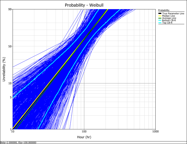
Create another SimuMatic folio and generate a second data using the same settings, but this time, select the RRY analysis method on the Analysis tab. The following plot shows the result.
The following plot shows the results using the MLE analysis method.
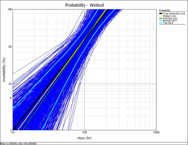
The results clearly demonstrate that the median RRX estimate provides the least deviation from the truth for this sample size and data type. However, the MLE outputs are grouped more closely together, as evidenced by the bounds.
This experiment can be repeated in SimuMatic using multiple censoring schemes (including Type I and Type II right censoring as well as random censoring) with various distributions. Multiple experiments can be performed with this utility to evaluate assumptions about the appropriate parameter estimation method to use for data sets.