MTTF, MTBF, Mean Time Between Replacements and MTBF with Scheduled Replacements
[Editor's Note: This article has been updated since its original publication to reflect a more recent version of the software interface.]
Seasoned reliability engineers know that there is a great deal of discussion and confusion regarding the terms MTTF and MTBF. We certainly hope that the addition of two more terms in the title won't scare readers away! In fact, the purpose of this article is to clear up the confusion by defining these terms and using examples to illustrate their differences and discuss the applications of each term. ReliaSoft's Weibull++, RGA and BlockSim software packages will be used for illustration.
MTTF: Mean time to failure describes the expected time to failure for a non-repairable system.
For example, assume you tested 3 identical systems starting from time 0 until all of them failed. The first system failed at 10 hours, the second failed at 12 hours and the third failed at 13 hours. The MTTF is the average of the three failure times, which is 11.6667 hours.
If these three failures are
random samples from a population and the failure times of this
population follow a distribution with a probability density
function (pdf) of
![]() , then
the population MTTF can be mathematically calculated by:
, then
the population MTTF can be mathematically calculated by:
|
|
(1) |
Assuming the failure times follow a Weibull distribution, we can use Weibull++ to estimate the parameters for the distribution and calculate the population MTTF. The analysis settings and estimated parameters are:
Table 1:
Results from Weibull++
| Distribution | Weibull-2P |
| Analysis | RRX |
| CB-Method | FM |
| Ranking | MED |
| Beta | 7.2393 |
| Eta | 12.3559 |
| Rho | 0.9904 |
| LK-Value | -5.2592 |
| Fail/Susp | 3/0 |
The Mean Life (MTTF) can be calculated in the Quick Calculation Pad (QCP):

Figure 1: MTTF Calculated in Weibull++
Figure 1 also gives the two-sided 90% confidence bounds of the estimated MTTF. The units of the calculated MTTF and its bound are the same as the units of time for the data (which happen to be hours in this example).
MTBDE: Mean Time between Downing Event, describes the expected time between two consecutive downing events for a repairable system.
For example, assume you are testing a system that can be repaired when there is a failure. The failures causes the system to go down. The first failure happens at 10 hours and it takes 5 hours to fix. The second failure is at 27 hours and the repair duration is 3 hours. Then after working for 13 hours, the system fails at 43 hours. The repair lasts for 7 hours and the system is restored at 50 hours. This failure and repair process can be illustrated using the following graph.

Figure 2: Failure and Repair Process for a Repairable System
without Scheduled Replacements
The MTBDE = x (T1 + T2) = 16.5 hours, if you use only the observations of complete cycles. You can add one more cycle by combining x0 and y3. Then the MTBDE = ⅓ x (T1 + T2 + x0 + y3) hours.
If all the uptime durations xi are independent and identically distributed (i.i.d) and all the repair durations yi are i.i.d, then:
|
MTBDE = MTBF + MTTR (Mean Time to Repair) |
(2) |
Eqn. (2) shows that the MTBDE is the sum of the average uptime and the average downtime (MTTR). The definition of MTBF is given next.
MTBF: Mean Time between Failures. This average time excludes the time spent waiting for repair, being repaired, being re-qualified, and other downing events such as inspections and preventive maintenance and so on; it is intended to measure only the time a system is available and operating.
For the above example, it will be:
MTBF = ⅓ (x0 + x1 + x2) = 11.6667
The above equation assumes that all the downing events are caused by failures. The duration of the downing events are the duration of repairs.
Again, this calculation assumes the uptime durations xi are i.i.d. However, for a repairable system, the i.i.d assumption for xi is rarely true unless the system can be treated as brand new after each repair or the distribution of xi is exponential. When the i.i.d assumption is not true (for example, for a non-homogenous Poisson process [NHPP]), MTBF is a function of time. Often, the repair duration is relatively short compared to the time between failures and can be ignored. ReliaSoft's RGA software package can be used to calculate MTBF for a repairable system when the repair durations are ignored. For example, a typical MTBF vs. Time plot in RGA will be:
Figure 3: MTBF vs. Time Plot
for a Repairable System
The points on the plot are the observed cumulative MTBFs. These values are calculated by the following equation:
|
|
(3) |
where:
-
t is the cumulative operating time.
-
N(t) is the observed number of failures by time t.
The curve in Figure 3 is the estimated MTBF by the Crow AMSAA model for repairable systems.
Mean Time Between Replacements: This metric is usually used for non-repairable components or subsystems in a repairable system. For example, a light bulb in a machine is replaced after every Tp hours of operation or replaced at failure. The mean time between replacements metric describes the average time between two consecutive replacements under these conditions.
If the replacement time is short and can be ignored, there is a closed form solution for mean time between replacements. The expected time between two adjacent replacements is given by:
|
|
(4) |
The first term in the above equation is for the case when the replacement occurs at the scheduled interval Tp. The second term is for the case when the replacement occurs at the first failure time x (0 < x < Tp ).
For example, if the light bulb has a Weibull distribution with β = 1.5, η = 5000 and Tp = 3000, the mean time between replacements is 2515, calculated by Eqn. (4). You also can use ReliaSoft's BlockSim to estimate this value through simulation. Since the replacement duration is ignored in Eqn. (4), it is set to a small number, such as 0.0001, in the simulation. The simulation settings are shown next.
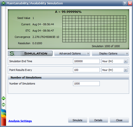
Figure 4: Simulation Settings in BlockSim
The simulation results are:
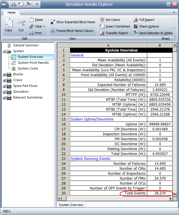
Figure 5: Simulation Results in BlockSim
From the results, we can see that the total number of events (replacements) is 39.274. The simulation time is 100,000. Therefore, the mean time between replacements is:
Mean Time between Replacements = 100,000/39.274 = 2546
This simulation result is close to the analytical solution, 2515.
MTBF with Scheduled Replacements (MTBF_SR): This metric is used in the same situations as mean time between replacements, but describes something different. Usually, it is used for non-repairable components or subsystems in a repairable system. For example, a light bulb in a system is replaced every Tp hours of working or replaced at failures. This metric describes the average time between two consecutive failures under these conditions.
For example, a failure and replacement process is given in Figure 6.
Figure 6: Failure and Replacement Process for a System with
Scheduled Replacements
In Figure 6, T1 is the time to the first failure, T2 is the duration between failure 1 and 2 and T3 is the duration between failure 2 and 3. The MTBF_SR is the average of these three values.
The MTBF with Scheduled Replacements metric also has a closed form solution if the replacement time is small enough that it can be ignored. The formula is:
|
|
(5) |

For the example used in the previous section, the MTBF with scheduled replacements is 6766, calculated from Eqn. (5). From the simulation results shown in Figure 5, we know that the number of failures is 14.695. So the mean time between failures with scheduled replacements can be calculated as:
MTBF with Scheduled Replacements = 100,000/14.695 = 6805
This result is close to the analytical solution, 6766. If you increase the number of simulations and use a larger simulation end time, you will get a result that is even closer to the analytical solution.
When there are multiple replaceable subsystems with different scheduled replacement intervals, it is not easy to find a closed form solution for MTBF_SR and mean time between replacements for the whole system. Using simulation is a better choice. MTBF_SR and mean time between replacements can be used to evaluate whether or not the scheduled replacement intervals are good. With other information, such as the logistic delays, crew costs and part costs, you can find an optimum replacement interval.
Conclusion
In this article, four commonly-used terms in reliability
engineering are discussed. Examples show how they are used for
different purposes. MTTF is usually used for non-repairable
systems. MTBF, the most well-known term, is usually used for
repairable systems and is also widely used for the case where
the failure distribution is exponential. Mean time between
replacements and MTBF with scheduled replacements are applied to
repairable systems with scheduled preventive maintenance. Mean
time between replacements can be used to find the optimum
maintenance interval to minimize the cost per unit time. For
details, please read
https://help.reliasoft.com/reference/system_analysis/sa/introduction_to_repairable_systems.html#PreventiveMaintenance1.