Software Reliability Growth Modeling Using the Standard and Modified Gompertz Models

[Editor's Note: This article has been updated since its original publication to reflect a more recent version of the software interface.]

Software reliability modeling and prediction during product development is an area of reliability that is getting more focus from software developers. The use of software reliability growth models plays an important role in measuring improvements, achieving effective and efficient test/debug scheduling during the course of a software development project, determining when to release a product or estimating the number of service releases required after release to reach a reliability goal. Many new trends in software development process standardization, in addition to established ones, emphasize the need for statistical metrics in monitoring reliability and quality improvements. In this article, we investigate the standard Gompertz and modified Gompertz models and show their applications in modeling software reliability growth using RGA.

There are essentially two approaches to performing statistical reliability prediction for software. The first approach, based on design parameters, estimates the number of defects in the software using code characteristics such as numbers of lines of code, nesting of loops, external references, input/output calls, etc. The second approach is reliability growth analysis based on statistical correlations of actual defect detection data obtained during testing. Many models are used to describe reliability growth in software such as Crow-AMSAA, standard Gompertz, modified Gompertz and Lloyd-Lipow.*

This article addresses the techniques available for the second approach using the Gompertz reliability growth models. Let us start with an overview of the basics of the Gompertz model and the modified Gompertz models. Then, we will discuss the application of these models for software development.

The Standard Gompertz Model

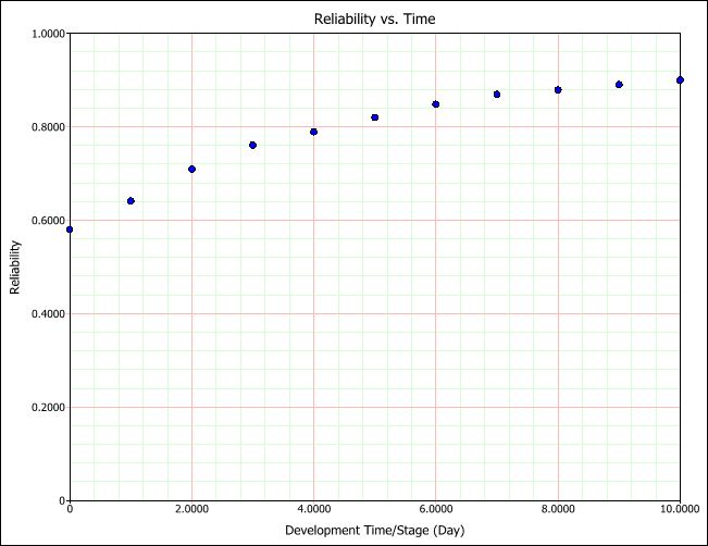
The standard Gompertz reliability growth model is often used when analyzing success/failure data and reliability data obtained in developmental reliability growth programs (the previous two issues of the Reliability HotWire, Issues 82 and 83, discussed reliability and success/failure data and other reliability growth models that can be used to model them). The standard Gompertz model is most applicable when the reliability data follow a concave shape, as shown in the next figure.

The standard Gompertz model is mathematically given by the following 3-parameter equation:

where:

T: time, launch number or stage number, T > 0
R: the system's reliability at T.
a: the upper limit that the reliability approaches asymptotically as T ∞, or the maximum reliability that can be attained.
ab: initial reliability at T = 0.
c: the growth pattern indicator (small values of c indicate rapid early reliability growth and large values of c indicate slow reliability growth).

The estimated parameters in RGA are unitless. The solution for the parameters, given Ti and Ri, is accomplished by fitting the best possible line through the data points. Many methods are available, all of which tend to be numerically intensive. For more details about the parameter estimation method used in RGA, click here.

The Modified Gompertz Model

Sometimes reliability growth data with an S-shaped trend, such as the one shown in the next figure, cannot be described accurately by the standard Gompertz or logistic curves. Since these two models have fixed values of reliability at the inflection points, only a few reliability growth data sets following an S-shaped reliability growth curve can be fitted to them. A modification of the standard Gompertz curve overcomes this shortcoming by considering a shift in the vertical coordinate:

where:

T: time, launch number or stage number, T > 0.
R: system's reliability at T.
d: shift parameter.
d + a: upper limit that the reliability approaches asymptotically as T ∞.
d + ab: initial reliability at T = 0.
c: growth pattern indicator (small values of c indicate rapid early reliability growth and large values of c indicate slow growth.

The Reliability vs. Time plot for this model looks like the figure shown next.

The parameters of the modified Gompertz model can be estimated using linear regression and confidence bounds can also be estimated; for more details about how to estimate confidence bounds, click here.

Many scenarios can be modeled with the S-shape behavior of the modified Gompertz. The S-shape behavior essentially distinguishes between multiple "phases" in the product reliability growth program. In the beginning of testing (first phase), scarcity in discovering problems and delays in identifying fixes can cause the improvement in reliability to be small. During the second phase, fixes become available and, with any additional discovered failures and implemented fixes, significant improvements are observed and the reliability grows at a fast pace. In the third phase, fewer and fewer failure modes are uncovered, as most of the failure modes have already been discovered. In addition, the reliability growth program might start running into limitations of technology and design that slow down the reliability growth.

Application to Software Reliability Growth

The standard and modified Gompertz models are praised for their simplicity and ability to produce valid estimates of the future reliability of the software and to provide estimates sufficiently early in the testing/debugging phase. The standard Gompertz model can be a good model to use in software reliability growth in cases where the bugs are discovered fairly early and improvements are made swiftly. The modified Gompertz model, on the other hand, is more appropriate to describe an S-shaped reliability growth curve trend with a lower rate of debugging and growth at the early stage, a higher rate later on as more fixes are found and successfully implemented, and ending with a slower rate of debugging toward the completion of the program, where the law of diminishing marginal returns causes slower improvements to the software. Time, in the standard and modified Gompertz models, can be represented by accumulated execution time, stages, accumulated CPU time, accumulated clock time or calendar time. Defect data can be represented in the form of a tally of discovered bugs, mean time between new discovered bugs, number of test cases and failed tests, etc.

Example 1

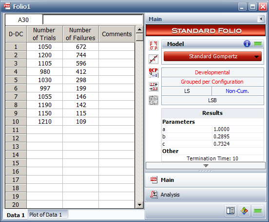
A software development company tracks the number of discovered bugs during the development of a new software application. The following figure shows the record of bugs discovered during 10 stages of the development cycle. Each stage consists of a number of performed tests (about 1100 tests) and the number of tests that failed the test. At the end of each stage, fixes are implemented in the software and a new version is compiled for the next stage of testing. This figure also shows the calculated parameters for the standard Gompertz model.

The next plot shows the estimated reliability plot along with the lower 90% one-sided confidence bound.

The next figure shows the calculation of the demonstrated reliability at the end of the test (10th stage of testing) with a 90% lower confidence estimate.

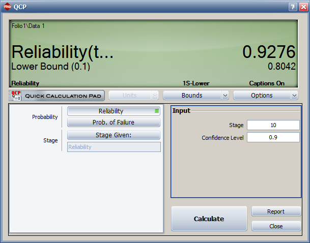
Because the "a" parameter in the standard Gompertz model is equal to 1, the testing/debugging program has the potential to grow the reliability of the software further than what is currently demonstrated. To achieve a reliability goal of 99%, for example, about 6.46 more stages of testing would be required.

Example 2

A software development company follows a process called the Capability Maturity Model (CMM), which is a process used in software development for controlling improvements and achieving high software quality. Like many other software development and quality assurance initiatives, CMM emphasizes statistical analysis to quantify and control the improvement process. The CMM process has different levels. To achieve Levels 4 and 5 of CMM, the company must set quantitative quality goals for the software product and measure and control its improvement using statistical techniques. The company is using reliability growth models to monitor and measure the software reliability.

In the current software development project, the company experienced slow growth at the initial testing stages, which relied on random exploratory testing. It was then able to improve the efficiency of the testing cases after better identification of the user profile and risk areas in the software. The last few stages of testing revealed software faults at a slower rate and the company expects that the software is reaching its maturity.

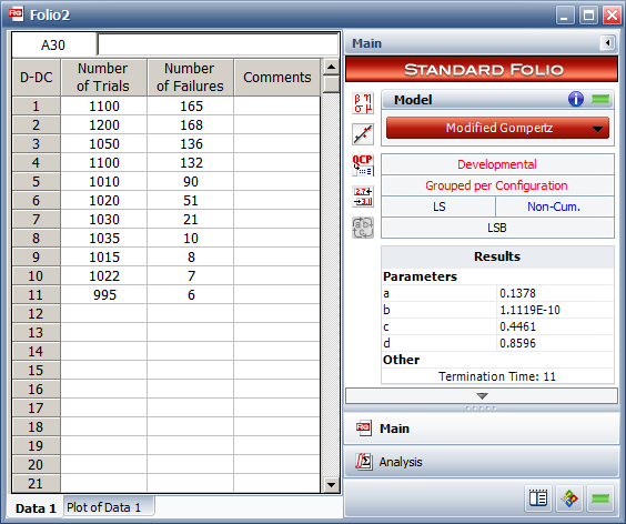
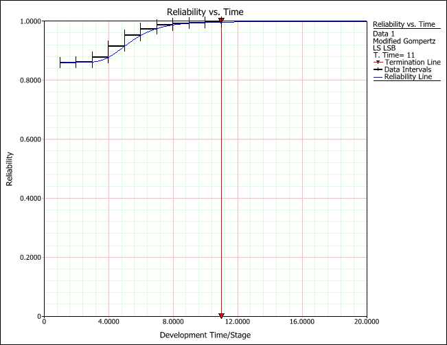
The following data set, shown entered in RGA, shows the test case results obtained at each of 11 stages of testing. The standard Gompertz model and the modified Gompertz model were fitted to the data set. The modified Gompertz model was a more appropriate model for this data set.

The reliability growth plot is shown next.

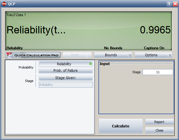
The achieved reliability is 0.9965, as shown next.

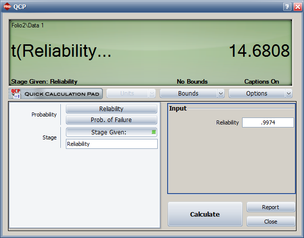
The asymptotic limit based on this reliability growth program is a + d = 0.9974. That reliability level is estimated to be achieved after about three stages of testing (at the 14.68th stage), as shown next.

Final Comments

Readers interested in seeing an additional software reliability growth application may wish to examine this case study.

*Other common models include Musa, Goel-Okumoto, Pareto and Yamada