
Gompertz Models
This chapter discusses the two Gompertz models that are used in Weibull++: the standard Gompertz and the modified Gompertz.
The Standard Gompertz Model
The Gompertz reliability growth model is often used when analyzing reliability data. It is most applicable when the data set follows a smooth curve, as shown in the plot below.
The Gompertz model is mathematically given by Virene [1]:


where:


 the system's reliability at development time, launch number or stage number,

 the upper limit that the reliability approaches asymptotically as
 , or the maximum reliability that can be attained
 initial reliability at

 the growth pattern indicator (small values of
 indicate rapid early reliability growth and large values of
 indicate slow reliability growth)


As it can be seen from the mathematical definition, the Gompertz model is a 3-parameter model with the parameters
 ,
,
 and
and
 . The solution for the parameters, given
 and
and
 , is accomplished by fitting the best possible line through the data points. Many methods are available; all of which tend to be numerically intensive. When analyzing reliability data in the Weibull++ software, you have the option to enter the reliability values in percent or in decimal format. However,
 will always be returned in decimal format and not in percent. The estimated parameters in the Weibull++ software are unitless. The next section presents an overview and background on some of the most commonly used algorithms/methods for obtaining these parameters.


Parameter Estimation
Linear Regression
The method of least squares requires that a straight line be fitted to a set of data points. If the regression is on
 , then the sum of the squares of the vertical deviations from the points to the line is minimized. If the regression is on
 , the line is fitted to a set of data points such that the sum of the squares of the horizontal deviations from the points to the line is minimized. To illustrate the method, this section presents a regression on
 . Consider the linear model given by Seber and Wild
[2]:
. Consider the linear model given by Seber and Wild
[2]:


or in matrix form where bold letters indicate matrices:


where:

![{\displaystyle Y=\left[{\begin{matrix}{{Y}_{1}}\\{{Y}_{2}}\\\vdots \\{{Y}_{N}}\\\end{matrix}}\right]\,\!}](https://en.wikipedia.org/api/rest_v1/media/math/render/svg/3886e601d4bc4b9d008d053685829d0d9f0980e6)

![{\displaystyle X=\left[{\begin{matrix}1&{{X}_{1,1}}&\cdots &{{X}_{1,p}}\\1&{{X}_{2,1}}&\cdots &{{X}_{2,p}}\\\vdots &\vdots &\ddots &\vdots \\1&{{X}_{N,1}}&\cdots &{{X}_{N,p}}\\\end{matrix}}\right]\,\!}](https://en.wikipedia.org/api/rest_v1/media/math/render/svg/152fed6c432b5d699820e40932d6fca8cb8403ef)
and:

![{\displaystyle \beta =\left[{\begin{matrix}{{\beta }_{0}}\\{{\beta }_{1}}\\\vdots \\{{\beta }_{p}}\\\end{matrix}}\right]\,\!}](https://en.wikipedia.org/api/rest_v1/media/math/render/svg/1d2e4dd282094c746a50cb055693fe76631babbf)
The vector  holds the values of the parameters. Now let
 be the estimates of these parameters, or the regression coefficients. The vector of estimated regression coefficients is denoted by:


![{\displaystyle {\widehat {\beta }}=\left[{\begin{matrix}{{\widehat {\beta }}_{0}}\\{{\widehat {\beta }}_{1}}\\\vdots \\{{\widehat {\beta }}_{p}}\\\end{matrix}}\right]\,\!}](https://en.wikipedia.org/api/rest_v1/media/math/render/svg/4957a32f327fd533a37732028d0cded85edd1fce)
Solving for  in the matrix form of the equation requires the analyst to left multiply both sides by the transpose of
 ,
,
 , or :


Now the term  becomes a square and invertible matrix. Then taking it to the other side of the equation gives:


Non-linear Regression
Non-linear regression is similar to linear regression, except that a curve is fitted to the data set instead of a straight line. Just as in the linear scenario, the sum of the squares of the horizontal and vertical distances between the line and the points are to be minimized. In the case of the non-linear Gompertz model
 , let:


where:

![{\displaystyle {{T}_{i}}=\left[{\begin{matrix}{{T}_{1}}\\{{T}_{2}}\\\vdots \\{{T}_{N}}\\\end{matrix}}\right],\quad i=1,2,...,N\,\!}](https://en.wikipedia.org/api/rest_v1/media/math/render/svg/46af4a1d7c85f39c62928b4fc8b6c3c02c43add3)
and:

![{\displaystyle \delta =\left[{\begin{matrix}a\\b\\c\\\end{matrix}}\right]\,\!}](https://en.wikipedia.org/api/rest_v1/media/math/render/svg/35288be38cbfc3ce3a56ad68d85aa1eb8cbd3717)
The Gauss-Newton method can be used to solve for the parameters
 ,
,
 and
and
 by performing a Taylor series expansion on
 Then approximate the non-linear model with linear terms and employ ordinary least squares to estimate the parameters. This procedure is performed in an iterative manner and it generally leads to a solution of the non-linear problem.

This procedure starts by using initial estimates of the parameters
 ,
,
 and
and
 , denoted as

 and
and
 where
where
 is the iteration number. The Taylor series expansion approximates the mean response,
 , around the starting values,

 and
and
 For the
 observation:


![{\displaystyle f({{T}_{i}},\delta )\simeq f({{T}_{i}},{{g}^{(0)}})+{\underset {k=1}{\overset {p}{\mathop {\sum } }}}\,{{\left[{\frac {\partial f({{T}_{i}},\delta )}{\partial {{\delta }_{k}}}}\right]}_{\delta ={{g}^{(0)}}}}({{\delta }_{k}}-g_{k}^{(0)})\,\!}](https://en.wikipedia.org/api/rest_v1/media/math/render/svg/8f5b9a09f1ee18b1d925d36a2437bd5990d564bd)
where:

![{\displaystyle {{g}^{(0)}}=\left[{\begin{matrix}g_{1}^{(0)}\\g_{2}^{(0)}\\g_{3}^{(0)}\\\end{matrix}}\right]\,\!}](https://en.wikipedia.org/api/rest_v1/media/math/render/svg/134742bde7505b007980fa188606324f84386edf)
Let:

![{\displaystyle {\begin{aligned}f_{i}^{(0)}=&f({{T}_{i}},{{g}^{(0)}})\\\nu _{k}^{(0)}=&({{\delta }_{k}}-g_{k}^{(0)})\\D_{ik}^{(0)}=&{{\left[{\frac {\partial f({{T}_{i}},\delta )}{\partial {{\delta }_{k}}}}\right]}_{\delta ={{g}^{(0)}}}}\end{aligned}}\,\!}](https://en.wikipedia.org/api/rest_v1/media/math/render/svg/bb23378999334f2771d9f0a6016e855e72e37ece)
So the equation  becomes:


or by shifting  to the left of the equation:


In matrix form this is given by:


where:

![{\displaystyle {{Y}^{(0)}}=\left[{\begin{matrix}{{Y}_{1}}-f_{1}^{(0)}\\{{Y}_{2}}-f_{2}^{(0)}\\\vdots \\{{Y}_{N}}-f_{N}^{(0)}\\\end{matrix}}\right]=\left[{\begin{matrix}{{Y}_{1}}-g_{1}^{(0)}g_{2}^{(0)g_{3}^{(0){{T}_{1}}}}\\{{Y}_{1}}-g_{1}^{(0)}g_{2}^{(0)g_{3}^{(0){{T}_{2}}}}\\\vdots \\{{Y}_{N}}-g_{1}^{(0)}g_{2}^{(0)g_{3}^{(0){{T}_{N}}}}\\\end{matrix}}\right]\,\!}](https://en.wikipedia.org/api/rest_v1/media/math/render/svg/8ae0fdf0707910fe67c213a1d30418881d739e3a)

![{\displaystyle {\begin{aligned}{{D}^{(0)}}=&\left[{\begin{matrix}D_{11}^{(0)}&D_{12}^{(0)}&D_{13}^{(0)}\\D_{21}^{(0)}&D_{22}^{(0)}&D_{23}^{(0)}\\.&.&.&.\\.&.&.&.\\D_{N1}^{(0)}&D_{N2}^{(0)}&D_{N3}^{(0)}\\\end{matrix}}\right]\\=&\left[{\begin{matrix}g_{2}^{(0)g_{3}^{(0){{T}_{1}}}}&{\tfrac {g_{1}^{(0)}}{g_{2}^{(0)}}}g_{3}^{(0){{T}_{1}}}g_{2}^{(0)g_{3}^{(0){{T}_{1}}}}&{\tfrac {g_{1}^{(0)}}{g_{3}^{(0)}}}g_{3}^{(0){{T}_{1}}}\ln(g_{2}^{(0)}){{T}_{1}}g_{2}^{(0)g_{3}^{(0){{T}_{1}}}}&1\\g_{2}^{(0)g_{3}^{(0){{T}_{2}}}}&{\tfrac {g_{1}^{(0)}}{g_{2}^{(0)}}}g_{3}^{(0){{T}_{2}}}g_{2}^{(0)g_{3}^{(0){{T}_{2}}}}&{\tfrac {g_{1}^{(0)}}{g_{3}^{(0)}}}g_{3}^{(0){{T}_{2}}}\ln(g_{2}^{(0)}){{T}_{2}}g_{2}^{(0)g_{3}^{(0){{T}_{2}}}}&1\\.&.&.&.\\.&.&.&.\\g_{2}^{(0)g_{3}^{(0){{T}_{N}}}}&{\tfrac {g_{1}^{(0)}}{g_{2}^{(0)}}}g_{3}^{(0){{T}_{N}}}g_{2}^{(0)g_{3}^{(0){{T}_{N}}}}&{\tfrac {g_{1}^{(0)}}{g_{3}^{(0)}}}g_{3}^{(0){{T}_{N}}}\ln(g_{2}^{(0)}){{T}_{N}}g_{2}^{(0)g_{3}^{(0){{T}_{N}}}}&1\\\end{matrix}}\right]\end{aligned}}\,\!}](https://en.wikipedia.org/api/rest_v1/media/math/render/svg/07563dd1204d5feadf9db630858e3b66e3708bf0)
and:

![{\displaystyle {{\nu }^{(0)}}=\left[{\begin{matrix}g_{1}^{(0)}\\g_{2}^{(0)}\\g_{3}^{(0)}\\\end{matrix}}\right]\,\!}](https://en.wikipedia.org/api/rest_v1/media/math/render/svg/0583937a9598920c2ce97b6ee4b749b7e6f6c89b)
Note that the equation  is in the form of the general linear regression model given in the
Linear Regression section. Therefore, the estimate of the parameters
is in the form of the general linear regression model given in the
Linear Regression section. Therefore, the estimate of the parameters
 is given by:


The revised estimated regression coefficients in matrix form are:


The least squares criterion measure,
 should be checked to examine whether the revised regression coefficients will lead to a reasonable result. According to the Least Squares Principle, the solution to the values of the parameters are those values that minimize
 . With the starting coefficients,
 ,
,
 is:
is:


![{\displaystyle {{Q}^{(0)}}={\underset {i=1}{\overset {N}{\mathop {\sum } }}}\,{{\left[{{Y}_{i}}-f\left({{T}_{i}},{{g}^{(0)}}\right)\right]}^{2}}\,\!}](https://en.wikipedia.org/api/rest_v1/media/math/render/svg/dea6cd91906cff93ccb13019648812e2156bb17d)
And with the coefficients at the end of the first iteration,
 ,
,
 is:
is:


![{\displaystyle {{Q}^{(1)}}={\underset {i=1}{\overset {N}{\mathop {\sum } }}}\,{{\left[{{Y}_{i}}-f\left({{T}_{i}},{{g}^{(1)}}\right)\right]}^{2}}\,\!}](https://en.wikipedia.org/api/rest_v1/media/math/render/svg/a2769160953f180f54f4cd225bf8b4d18265c549)
For the Gauss-Newton method to work properly and to satisfy the Least Squares Principle, the relationship
 has to hold for all
 , meaning that
 gives a better estimate than
 . The problem is not yet completely solved. Now
 are the starting values, producing a new set of values
 . The process is continued until the following relationship has been satisfied:


When using the Gauss-Newton method or some other estimation procedure, it is advisable to try several sets of starting values to make sure that the solution gives relatively consistent results.
Choice of Initial Values
The choice of the starting values for the nonlinear regression is not an easy task. A poor choice may result in a lengthy computation with many iterations. It may also lead to divergence, or to a convergence due to a local minimum. Therefore, good initial values will result in fast computations with few iterations, and if multiple minima exist, it will lead to a solution that is a minimum.
Various methods were developed for obtaining valid initial values for the regression parameters. The following procedure is described by Virene [1] in estimating the Gompertz parameters. This procedure is rather simple. It will be used to get the starting values for the Gauss-Newton method, or for any other method that requires initial values. Some analysts use this method to calculate the parameters when the data set is divisible into three groups of equal size. However, if the data set is not equally divisible, it can still provide good initial estimates.
Consider the case where  observations are available in the form shown next. Each reliability value,
 , is measured at the specified times,
 .
.


where:

 is equal to the number of items in each equally sized group


The Gompertz reliability equation is given by:

and:


Define:


Then:


Without loss of generality, take  ; then:


Solving for  yields:


Considering the definitions for  and
and
 , given above, then:


or:


Reordering the equation yields:

![{\displaystyle {\begin{aligned}\ln(a)=&{\frac {1}{n}}\left({{S}_{1}}+{\frac {{{S}_{2}}-{{S}_{1}}}{1-{{c}^{n\cdot I}}}}\right)\\a=&{{e}^{\left[{\tfrac {1}{n}}\left({{S}_{1}}+{\tfrac {{{S}_{2}}-{{S}_{1}}}{1-{{c}^{n\cdot I}}}}\right)\right]}}\end{aligned}}\,\!}](https://en.wikipedia.org/api/rest_v1/media/math/render/svg/3b669066ed702b1061c256f92fc3be2a6f19eecc)
If the reliability values are in percent then
 needs to be divided by 100 to return the estimate in decimal format. Consider the definitions for
 and
and
 again, where:


Reordering the equation above yields:

![{\displaystyle {\begin{aligned}\ln(b)=&{\frac {({{S}_{2}}-{{S}_{1}})({{c}^{I}}-1)}{{(1-{{c}^{n\cdot I}})}^{2}}}\\b=&{{e}^{\left[{\tfrac {\left({{S}_{2}}-{{S}_{1}}\right)\left({{c}^{I}}-1\right)}{{\left(1-{{c}^{n\cdot I}}\right)}^{2}}}\right]}}\end{aligned}}\,\!}](https://en.wikipedia.org/api/rest_v1/media/math/render/svg/5ca2f57b03f98f53d813ca64261a984aa717027d)
Therefore, for the special case where
 , the parameters are:


![{\displaystyle {\begin{aligned}c=&{{\left({\frac {{{S}_{3}}-{{S}_{2}}}{{{S}_{2}}-{{S}_{1}}}}\right)}^{\tfrac {1}{n}}}\\a=&{{e}^{\left[{\tfrac {1}{n}}\left({{S}_{1}}+{\tfrac {{{S}_{2}}-{{S}_{1}}}{1-{{c}^{n}}}}\right)\right]}}\\b=&{{e}^{\left[{\tfrac {({{S}_{2}}-{{S}_{1}})(c-1)}{{\left(1-{{c}^{n}}\right)}^{2}}}\right]}}\end{aligned}}\,\!}](https://en.wikipedia.org/api/rest_v1/media/math/render/svg/46614b5c4b624e4de9295e9fd15903304ab28b0c)
To estimate the values of the parameters
 and
and
 , do the following:

- Arrange the currently available data in terms of
 and
and
 as in the table below. The
 values should be chosen at equal intervals and increasing in value by 1, such as one month, one hour, etc.
Design and Development Time vs. Demonstrated Reliability Data for a Device Group Number Growth Time  (months)
Reliability  (%)
(%)
0 58 4.060 1 1 66 4.190  = 8.250
2 72.5 4.284 2 3 78 4.357  = 8.641
4 82 4.407 3 5 85 4.443  = 8.850
- Calculate the natural log
 .
.
- Divide the column of values for log
 into three groups of equal size, each containing
 items. There should always be three groups. Each group should always have the same number,
 , of items, measurements or values.
- Add the values of the natural log
 in each group, obtaining the sums identified as
 ,
,
 and
and
 , starting with the lowest values of the natural log
 .
.
- Calculate
 using the following equation:
- Calculate
 using the following equation:
- Calculate
 using the following equation:
- Write the Gompertz reliability growth equation.
- Substitute the value of
 , the time at which the reliability goal is to be achieved, to see if the reliability is indeed to be attained or exceeded by
 .
.


![{\displaystyle a={{e}^{\left[{\tfrac {1}{n}}\left({{S}_{1}}+{\tfrac {{{S}_{2}}-{{S}_{1}}}{1-{{c}^{n}}}}\right)\right]}}\,\!}](https://en.wikipedia.org/api/rest_v1/media/math/render/svg/ce021e92c3ae1fc54b2821b466d5b1f8a6a4b8c3)

![{\displaystyle b={{e}^{\left[{\tfrac {({{S}_{2}}-{{S}_{1}})(c-1)}{{\left(1-{{c}^{n}}\right)}^{2}}}\right]}}\,\!}](https://en.wikipedia.org/api/rest_v1/media/math/render/svg/a4455554e664d2cf748a636a428679b5b6e114ce)
Confidence Bounds
The approximate reliability confidence bounds under the Gompertz model can be obtained with non-linear regression. Additionally, the reliability is always between 0 and 1. In order to keep the endpoints of the confidence interval, the logit transformation is used to obtain the confidence bounds on reliability.

![{\displaystyle CB={\frac {{\hat {R}}_{i}}{{{\hat {R}}_{i}}+(1-{{\hat {R}}_{i}}){{e}^{\pm {{z}_{\alpha }}{{\hat {\sigma }}_{R}}/\left[{{\hat {R}}_{i}}(1-{{\hat {R}}_{i}})\right]}}}}\,\!}](https://en.wikipedia.org/api/rest_v1/media/math/render/svg/d88953235136a9f72072101755d4d193e75f95a1)


where  is the total number of groups (in this case 3) and
 is the total number of items in each group.

Example - Standard Gompertz for Reliability Data
A device is required to have a reliability of 92% at the end of a 12-month design and development period. The following table gives the data obtained for the first five moths.
- What will the reliability be at the end of this 12-month period?
- What will the maximum achievable reliability be if the reliability program plan pursued during the first 5 months is continued?
- How do the predicted reliability values compare with the actual values?
| Group Number | Growth Time  (months) (months) |
Reliability  (%) (%) |

|
|---|---|---|---|
| 0 | 58 | 4.060 | |
| 1 | 1 | 66 | 4.190 |
 = 8.250 = 8.250
|
|||
| 2 | 72.5 | 4.284 | |
| 2 | 3 | 78 | 4.357 |
 = 8.641 = 8.641
|
|||
| 4 | 82 | 4.407 | |
| 3 | 5 | 85 | 4.443 |
 = 8.850 = 8.850
|
Solution
After generating the table above and calculating the last column to find
 ,
,
 and
and
 , proceed as follows:
- Solve for the value of
 :
:
- Solve for the value of
 :
:
- This is the upper limit for the reliability as
 .
.
- Solve for the value of
 :
:


![{\displaystyle {\begin{aligned}a&=e^{\left[({{\frac {1}{2}}\left(8.250+{\frac {S_{2}-S_{1}}{1-c^{n\cdot 1}}}\right)}\right]}\\&=e^{4.545}\\&=94.16\%\end{aligned}}\,\!}](https://en.wikipedia.org/api/rest_v1/media/math/render/svg/9f7e278cc6dc58a6e7ff1df3c5884038becc7e5c)

![{\displaystyle {\begin{aligned}b=&{{e}^{\left[{\tfrac {(8.641-8.250)(0.731-1)}{{(1-{{0.731}^{2}})}^{2}}}\right]}}\\=&{{e}^{(-0.485)}}\\=&0.615\end{aligned}}\,\!}](https://en.wikipedia.org/api/rest_v1/media/math/render/svg/4a7d977a0713c35845e5fbc24e74414f3f78121b)
Now, that the initial values have been determined, the Gauss-Newton method can be used. Therefore, substituting


 become:


![{\displaystyle {{Y}^{(0)}}=\left[{\begin{matrix}0.0916\\0.0015\\-0.1190\\0.1250\\0.0439\\-0.0743\\\end{matrix}}\right]\,\!}](https://en.wikipedia.org/api/rest_v1/media/math/render/svg/88b55aa266d4e27db6bf6681a7dba71fb7ad9867)

![{\displaystyle {{D}^{(0)}}=\left[{\begin{matrix}0.6150&94.1600&0.0000\\0.7009&78.4470&-32.0841\\0.7712&63.0971&-51.6122\\0.8270&49.4623&-60.6888\\0.8704&38.0519&-62.2513\\0.9035&28.8742&-59.0463\\\end{matrix}}\right]\,\!}](https://en.wikipedia.org/api/rest_v1/media/math/render/svg/d1034681e1adce790219bf5ad7f035d6d5a59d3a)

![{\displaystyle {{\nu }^{(0)}}=\left[{\begin{matrix}g_{1}^{(0)}\\g_{2}^{(0)}\\g_{3}^{(0)}\\\end{matrix}}\right]=\left[{\begin{matrix}94.16\\0.615\\0.731\\\end{matrix}}\right]\,\!}](https://en.wikipedia.org/api/rest_v1/media/math/render/svg/001792742aa9b017bc57864be5c0f28ac41fabcd)
The estimate of the parameters  is given by:


The revised estimated regression coefficients in matrix form are:


If the Gauss-Newton method works effectively, then the relationship
 has to hold, meaning that
 gives better estimates than
 , after
 . With the starting coefficients,
 ,
,
 is:
is:

![{\displaystyle {\begin{aligned}Q^{0}&=\sum _{i=1}^{N}\left[Y_{i}-f\left(T_{i},g^{(0)}\right)\right]^{2}\\&=0.045622\end{aligned}}}](https://en.wikipedia.org/api/rest_v1/media/math/render/svg/15326538ad98c1b6c4cb03c6578bf0d0f8342edc)
And with the coefficients at the end of the first iteration,
 ,
,
 is:
is:

![{\displaystyle {\begin{aligned}Q^{1}&=\sum _{i=1}^{N}\left[Y_{i}-f\left(T_{i},g^{(1)}\right)\right]^{2}\\&=0.041439\end{aligned}}}](https://en.wikipedia.org/api/rest_v1/media/math/render/svg/e82269cc837ab915f5cbac5fb2058185ff0d1587)
Therefore, it can be justified that the Gauss-Newton method works in the right direction. The iterations are continued until the relationship
 is satisfied. Note that the Weibull++ software uses a different analysis method called the
Levenberg-Marquardt. This method utilizes the best features of the Gauss-Newton method and the method of the steepest descent, and occupies a middle ground between these two methods. The estimated parameters using Weibull++ are shown in the figure below.
is satisfied. Note that the Weibull++ software uses a different analysis method called the
Levenberg-Marquardt. This method utilizes the best features of the Gauss-Newton method and the method of the steepest descent, and occupies a middle ground between these two methods. The estimated parameters using Weibull++ are shown in the figure below.


They are:


The Gompertz reliability growth curve is:


- The achievable reliability at the end of the 12-month period of design and development is:
- The maximum achievable reliability from Step 2, or from the value of
 , is 0.9422.
- The predicted reliability values, as calculated from the standard Gompertz model, are compared with the actual data in the table below. It may be seen in the table that the Gompertz curve appears to provide a very good fit for the data used because the equation reproduces the available data with less than 1% error. The standard Gompertz model is plotted in the figure below the table. The plot identifies the type of reliability growth curve that the equation represents.
Comparison of the Predicted Reliabilities with the Actual Data Growth Time  (months)
Gompertz Reliability (%) Raw Data Reliability (%) 0 57.97 58.00 1 66.02 66.00 2 72.62 72.50 3 77.87 78.00 4 81.95 82.00 5 85.07 85.00 6 87.43 7 89.20 8 90.52 9 91.50 10 92.22 11 92.75 12 93.14 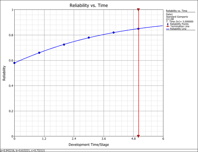


Example - Standard Gompertz for Sequential Data
Calculate the parameters of the Gompertz model using the sequential data in the following table.
| Run Number | Result | Successes | Observed Reliability (%) |
|---|---|---|---|
| 1 | F | 0 | |
| 2 | F | 0 | |
| 3 | F | 0 | |
| 4 | S | 1 | 25.00 |
| 5 | F | 1 | 20.00 |
| 6 | F | 1 | 16.67 |
| 7 | S | 2 | 28.57 |
| 8 | S | 3 | 37.50 |
| 9 | S | 4 | 44.44 |
| 10 | S | 5 | 50.00 |
| 11 | S | 6 | 54.55 |
| 12 | S | 7 | 58.33 |
| 13 | S | 8 | 61.54 |
| 14 | S | 9 | 64.29 |
| 15 | S | 10 | 66.67 |
| 16 | S | 11 | 68.75 |
| 17 | F | 11 | 64.71 |
| 18 | S | 12 | 66.67 |
| 19 | F | 12 | 63.16 |
| 20 | S | 13 | 65.00 |
| 21 | S | 14 | 66.67 |
| 22 | S | 15 | 68.18 |
Solution
Using Weibull++, the parameter estimates are shown in the following figure.

Cumulative Reliability
For many kinds of equipment, especially missiles and space systems, only success/failure data (also called discrete or attribute data) is obtained. Conservatively, the cumulative reliability can be used to estimate the trend of reliability growth. The cumulative reliability is given by Kececioglu [3]:


where:
 is the current number of trials
 is the number of failures


It must be emphasized that the instantaneous reliability of the developed equipment is increasing as the test-analyze-fix-and-test process continues. In addition, the instantaneous reliability is higher than the cumulative reliability. Therefore, the reliability growth curve based on the cumulative reliability can be thought of as the lower bound of the true reliability growth curve.
The Modified Gompertz Model
Sometimes, reliability growth data with an S-shaped trend cannot be described accurately by the Standard Gompertz or Logistic curves. Because these two models have fixed values of reliability at the inflection points, only a few reliability growth data sets following an S-shaped reliability growth curve can be fitted to them. A modification of the Gompertz curve, which overcomes this shortcoming, is given next [5].
If we apply a shift in the vertical coordinate, then the Gompertz model is defined by:


where:


 is the system's reliability at development time
 or at launch number
 , or stage number

 is the shift parameter
 is the upper limit that the reliability approaches asymptotically as

 is the initial reliability at

 is the growth pattern indicator (small values of
 indicate rapid early reliability growth and large values of
 indicate slow reliability growth)


The modified Gompertz model is more flexible than the original, especially when fitting growth data with S-shaped trends.
Parameter Estimation
To implement the modified Gompertz growth model, initial values of the parameters
 ,
,
 ,
,
 and
and
 must be determined. When analyzing reliability data in Weibull++, you have the option to enter the reliability values in percent or in decimal format. However,
 and
and
 will always be returned in decimal format and not in percent. The estimated parameters in W eibull++are unitless.
Given that  and
and
 , it follows that
 ,
,
 and
and
 , as defined in the derivation of the Standard Gompertz model, can be expressed as functions of
 .
.


Modifying the equations for estimating parameters
 ,
,
 ,
,
 , as functions of
 , yields:

![{\displaystyle {\begin{aligned}c(d)=&{{\left[{\frac {{{S}_{3}}(d)-{{S}_{2}}(d)}{{{S}_{2}}(d)-{{S}_{1}}(d)}}\right]}^{\tfrac {1}{n\cdot I}}}\\a(d)=&{{e}^{\left[{\tfrac {1}{n}}\left({{S}_{1}}(d)+{\tfrac {{{S}_{2}}(d)-{{S}_{1}}(d)}{1-{{[c(d)]}^{n\cdot I}}}}\right)\right]}}\\b(d)=&{{e}^{\left[{\tfrac {\left[{{S}_{2}}(d)-{{S}_{1}}(d)\right]\left[{{[c(d)]}^{I}}-1\right]}{{\left[1-{{[c(d)]}^{n\cdot I}}\right]}^{2}}}\right]}}\end{aligned}}\,\!}](https://en.wikipedia.org/api/rest_v1/media/math/render/svg/f43b527b4be5df960b07ba1838fcd5173340979c)
where  is the time interval increment. At this point, you can use the initial constraint of:


Now there are four unknowns,  ,
,
 ,
,
 and
and
 , and four corresponding equations. The simultaneous solution of these equations yields the four initial values for the parameters of the modified Gompertz model. This procedure is similar to the one discussed before. It starts by using initial estimates of the parameters,
 ,
,
 ,
,
 and
and
 , denoted as


 and
and
 where
where
 is the iteration number.


The Taylor series expansion approximates the mean response,
 , around the starting values,


 and
and
 . For the
 observation:


![{\displaystyle f({{T}_{i}},\delta )\simeq f({{T}_{i}},{{g}^{(0)}})+{\underset {k=1}{\overset {p}{\mathop {\sum } }}}\,{{\left[{\frac {\partial f({{T}_{i}},\delta )}{\partial {{\delta }_{k}}}}\right]}_{\delta ={{g}^{(0)}}}}\cdot ({{\delta }_{k}}-g_{k}^{(0)})\,\!}](https://en.wikipedia.org/api/rest_v1/media/math/render/svg/3898ce46a25b796fd5d3239d56d4cc00c41fe43c)
where:

![{\displaystyle {{g}^{(0)}}=\left[{\begin{matrix}g_{1}^{(0)}\\g_{2}^{(0)}\\g_{3}^{(0)}\\g_{4}^{(0)}\\\end{matrix}}\right]\,\!}](https://en.wikipedia.org/api/rest_v1/media/math/render/svg/f72571040025370bc67cd4bd51591b4287755417)
Let:

Therefore:


or by shifting  to the left of the equation:


In matrix form, this is given by:

where:

![{\displaystyle {{Y}^{(0)}}=\left[{\begin{matrix}{{Y}_{1}}-f_{1}^{(0)}\\.\\.\\{{Y}_{N}}-f_{N}^{(0)}\\\end{matrix}}\right]=\left[{\begin{matrix}{{Y}_{1}}-g_{4}^{(0)}+g_{1}^{(0)}g_{2}^{(0)g_{3}^{(0){{T}_{1}}}}\\.\\.\\{{Y}_{N}}-g_{4}^{(0)}+g_{1}^{(0)}g_{2}^{(0)g_{3}^{(0){{T}_{N}}}}\\\end{matrix}}\right]\,\!}](https://en.wikipedia.org/api/rest_v1/media/math/render/svg/18e774c35a1ff8e7f38c4bef7187b3f4531ba35f)

![{\displaystyle {\begin{aligned}{{D}^{(0)}}=&\left[{\begin{matrix}D_{11}^{(0)}&D_{12}^{(0)}&D_{13}^{(0)}&D_{14}^{(0)}\\.&.&.&.\\.&.&.&.\\D_{N1}^{(0)}&D_{N2}^{(0)}&D_{N3}^{(0)}&D_{N4}^{(0)}\\\end{matrix}}\right]\\=&\left[{\begin{matrix}g_{2}^{(0)g_{3}^{(0){{T}_{1}}}}&{\tfrac {g_{1}^{(0)}}{g_{2}^{(0)}}}g_{3}^{(0){{T}_{1}}}g_{2}^{(0)g_{3}^{(0){{T}_{1}}}}&{\tfrac {g_{1}^{(0)}}{g_{3}^{(0)}}}g_{3}^{(0){{T}_{1}}}\ln(g_{2}^{(0)}){{T}_{1}}g_{2}^{(0)g_{3}^{(0){{T}_{1}}}}&1\\.&.&.&.\\.&.&.&.\\g_{2}^{(0)g_{3}^{(0){{T}_{N}}}}&{\tfrac {g_{1}^{(0)}}{g_{2}^{(0)}}}g_{3}^{(0){{T}_{N}}}g_{2}^{(0)g_{3}^{(0){{T}_{N}}}}&{\tfrac {g_{1}^{(0)}}{g_{3}^{(0)}}}g_{3}^{(0){{T}_{N}}}\ln(g_{2}^{(0)}){{T}_{N}}g_{2}^{(0)g_{3}^{(0){{T}_{N}}}}&1\\\end{matrix}}\right]\end{aligned}}\,\!}](https://en.wikipedia.org/api/rest_v1/media/math/render/svg/3ef5263ac7f37fdd8e855689b70b0f1c55a4eb28)

![{\displaystyle {{\nu }^{(0)}}=\left[{\begin{matrix}g_{1}^{(0)}\\g_{2}^{(0)}\\g_{3}^{(0)}\\g_{4}^{(0)}\\\end{matrix}}\right]\,\!}](https://en.wikipedia.org/api/rest_v1/media/math/render/svg/bf58867fcbda0574eb6e41939db6fd7c4563e8c7)
The same reasoning as before is followed here, and the estimate of the parameters
 is given by:

The revised estimated regression coefficients in matrix form are:

To see if the revised regression coefficients will lead to a reasonable result, the least squares criterion measure,
 , should be checked. According to the Least Squares Principle, the solution to the values of the parameters are those values that minimize
 . With the starting coefficients,
 ,
,
 is:
is:


With the coefficients at the end of the first iteration,
 ,
,
 is:
is:


For the Gauss-Newton method to work properly, and to satisfy the Least Squares Principle, the relationship
 has to hold for all
 , meaning that
 gives a better estimate than
 . The problem is not yet completely solved. Now
 are the starting values, producing a new set of values
 The process is continued until the following relationship has been satisfied.


As mentioned previously, when using the Gauss-Newton method or some other estimation procedure, it is advisable to try several sets of starting values to make sure that the solution gives relatively consistent results. Note that Weibull++ uses a different analysis method called the Levenberg-Marquardt. This method utilizes the best features of the Gauss-Newton method and the method of the steepest descent, and occupies a middle ground between these two methods.
Confidence Bounds
The approximate reliability confidence bounds under the modified Gompertz model can be obtained using non-linear regression. Additionally, the reliability is always between 0 and 1. In order to keep the endpoints of the confidence interval, the logit transformation can be used to obtain the confidence bounds on reliability.


where  is the total number of groups (in this case 4) and
 is the total number of items in each group.
Example - Modified Gompertz for Reliability Data
A reliability growth data set is given in columns 1 and 2 of the following table. Find the modified Gompertz curve that represents the data and plot it comparatively with the raw data.
| Time (months) | Raw Data Reliability (%) | Gompertz Reliability (%) | Logistic Reliability (%) | Modified Gompertz Reliability (%) |
|---|---|---|---|---|
| 0 | 31.00 | 25.17 | 22.70 | 31.18 |
| 1 | 35.50 | 38.33 | 38.10 | 35.08 |
| 2 | 49.30 | 51.35 | 56.40 | 49.92 |
| 3 | 70.10 | 62.92 | 73.00 | 69.23 |
| 4 | 83.00 | 72.47 | 85.00 | 83.72 |
| 5 | 92.20 | 79.94 | 93.20 | 92.06 |
| 6 | 96.40 | 85.59 | 96.10 | 96.29 |
| 7 | 98.60 | 89.75 | 98.10 | 98.32 |
| 8 | 99.00 | 92.76 | 99.10 | 99.27 |
Solution
To determine the parameters of the modified Gompertz curve, use:


![{\displaystyle c(d)={{\left[{\frac {{{S}_{3}}(d)-{{S}_{2}}(d)}{{{S}_{2}}(d)-{{S}_{1}}(d)}}\right]}^{\tfrac {1}{3}}}\,\!}](https://en.wikipedia.org/api/rest_v1/media/math/render/svg/f3f2027a28f8214620de0fb5d8224c762f873029)

![{\displaystyle a(d)={{e}^{\left[{\tfrac {1}{3}}\left({{S}_{1}}(d)+{\tfrac {{{S}_{2}}(d)-{{S}_{1}}(d)}{1-{{[c(d)]}^{3}}}}\right)\right]}}\,\!}](https://en.wikipedia.org/api/rest_v1/media/math/render/svg/6fea34af38c8d14f4cf11806e0fa05f7bad59516)

![{\displaystyle b(d)={{e}^{\left[{\tfrac {({{S}_{2}}(d)-{{S}_{1}}(d))(c(d)-1)}{{\left[1-{{[c(d)]}^{3}}\right]}^{2}}}\right]}}\,\!}](https://en.wikipedia.org/api/rest_v1/media/math/render/svg/3f5507c64e212e381cd478ba62ac765425c5e97f)
and:


for  , the equation above may be rewritten as:


The equations for parameters  ,
,
 and
and
 can now be solved simultaneously. One method for solving these equations numerically is to substitute different values of
 , which must be less than
 , into the last equation shown above, and plot the results along the y-axis with the value of
 along the x-axis. The value of
 can then be read from the x-intercept. This can be repeated for greater accuracy using smaller and smaller increments of
 . Once the desired accuracy on
 has been achieved, the value of
 can then be used to solve for
 ,
,
 and
and
 . For this case, the initial estimates of the parameters are:


Now, since the initial values have been determined, the Gauss-Newton method can be used. Therefore, substituting


 and
and
 ,
,

 become:


![{\displaystyle {{Y}^{(0)}}=\left[{\begin{matrix}0.000026\\0.253873\\-1.062940\\0.565690\\-0.845260\\0.096737\\0.076450\\0.238155\\-0.320890\\\end{matrix}}\right]\,\!}](https://en.wikipedia.org/api/rest_v1/media/math/render/svg/0fd4707e2f6f519d7e32831a10030b101357791d)

![{\displaystyle {{D}^{(0)}}=\left[{\begin{matrix}0.002524&69.3240&0.0000&1\\0.063775&805.962&-26.4468&1\\0.281835&1638.82&-107.552&1\\0.558383&1493.96&-147.068&1\\0.764818&941.536&-123.582&1\\0.883940&500.694&-82.1487&1\\0.944818&246.246&-48.4818&1\\0.974220&116.829&-26.8352&1\\0.988055&54.5185&-14.3117&1\\\end{matrix}}\right]\,\!}](https://en.wikipedia.org/api/rest_v1/media/math/render/svg/570a37ae57b3ef9c4e7d8498064fab7f87dd97f6)

![{\displaystyle {{\nu }^{(0)}}=\left[{\begin{matrix}g_{1}^{(0)}\\g_{2}^{(0)}\\g_{3}^{(0)}\\g_{4}^{(0)}\\\end{matrix}}\right]=\left[{\begin{matrix}69.324\\0.002524\\0.46012\\30.825\\\end{matrix}}\right]\,\!}](https://en.wikipedia.org/api/rest_v1/media/math/render/svg/985c4bdb0a0574de1de1d32a4c866fff85a1f848)
The estimate of the parameters  is given by:

![{\displaystyle {\begin{aligned}{{\widehat {\nu }}^{(0)}}=&{{\left({{D}^{{(0)}^{T}}}{{D}^{(0)}}\right)}^{-1}}{{D}^{{(0)}^{T}}}{{Y}^{(0)}}\\=&\left[{\begin{matrix}-0.275569\\-0.000549\\-0.003202\\0.209458\\\end{matrix}}\right]\end{aligned}}\,\!}](https://en.wikipedia.org/api/rest_v1/media/math/render/svg/e683d5445658b40c54244f6e9738a5e7ea5650b6)
The revised estimated regression coefficients in matrix form are given by:

![{\displaystyle {\begin{aligned}{{g}^{(1)}}=&{{g}^{(0)}}+{{\widehat {\nu }}^{(0)}}.\\=&\left[{\begin{matrix}69.324\\0.002524\\0.46012\\30.825\\\end{matrix}}\right]+\left[{\begin{matrix}-0.275569\\-0.000549\\-0.003202\\0.209458\\\end{matrix}}\right]\\=&\left[{\begin{matrix}69.0484\\0.00198\\0.45692\\31.0345\\\end{matrix}}\right]\end{aligned}}\,\!}](https://en.wikipedia.org/api/rest_v1/media/math/render/svg/d1d04df08a0f7eb0acd74403b10156c8761b10ca)
With the starting coefficients  ,
,
 is:
is:


With the coefficients at the end of the first iteration,
 ,
,
 is:
is:

![{\displaystyle {\begin{aligned}{{Q}^{(1)}}=&{\underset {i=1}{\overset {N}{\mathop {\sum } }}}\,{{\left[{{Y}_{i}}-f\left({{T}_{i}},{{g}^{(1)}}\right)\right]}^{2}}\\=&2.073964\end{aligned}}\,\!}](https://en.wikipedia.org/api/rest_v1/media/math/render/svg/cc8cf912f99efdf6d555cf175025184be5d8cf38)
Therefore:


Hence, the Gauss-Newton method works in the right direction. The iterations are continued until the relationship of
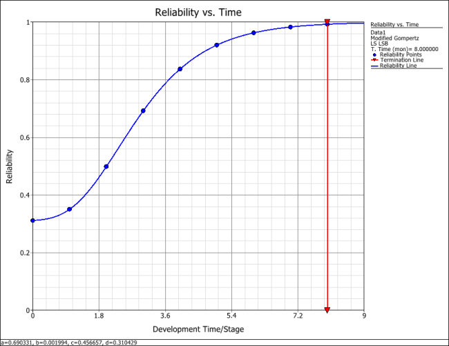
 has been satisfied. Using Weibull++RGA, the estimators of the parameters are:


Therefore, the modified Gompertz model is:


Using this equation, the predicted reliability is plotted in the following figure along with the raw data. As you can see, the modified Gompertz curve represents the data very well.
More Examples
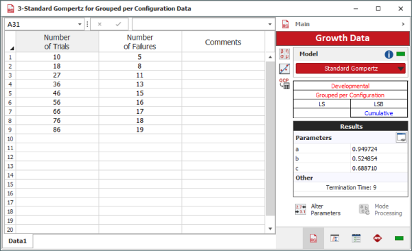
Standard Gompertz for Grouped per Configuration Data
A new design is put through a reliability growth test. The requirement is that after the ninth stage the design will exhibit an 85% reliability with a 90% confidence level. Given the data in the following table, do the following:
- Estimate the parameters of the standard Gompertz model.
- What is the initial reliability at
 ?
? - Determine the reliability at the end of the ninth stage and check to see whether the goal has been met.
| Stage | Number of Units | Number of Failures |
|---|---|---|
| 1 | 10 | 5 |
| 2 | 8 | 3 |
| 3 | 9 | 3 |
| 4 | 9 | 2 |
| 5 | 10 | 2 |
| 6 | 10 | 1 |
| 7 | 10 | 1 |
| 8 | 10 | 1 |
| 9 | 10 | 1 |
Solution
- The data is entered in cumulative format and the estimated standard Gompertz parameters are shown in the following figure.
- The initial reliability at
 is equal to:
- The reliability at the ninth stage can be calculated using the Quick Calculation Pad (QCP) as shown in the figure below.

The estimated reliability at the end of the ninth stage is equal to 94.97%. However, the lower limit at the 90% 1-sided confidence bound is equal to 85.2%. Therefore, the required goal of 85% reliability at a 90% confidence level has been met.


Comparing Standard and Modified Gompertz
Using the data in the following table, determine whether the standard Gompertz or modified Gompertz would be better suited for analyzing the given data.
| Stage | Reliability (%) |
|---|---|
| 0 | 36 |
| 1 | 38 |
| 2 | 46 |
| 3 | 58 |
| 4 | 71 |
| 5 | 80 |
| 6 | 86 |
| 7 | 88 |
| 8 | 90 |
| 9 | 91 |
Solution
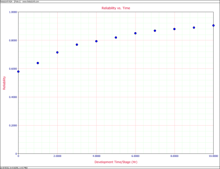
The standard Gompertz Reliability vs. Time plot is shown next.
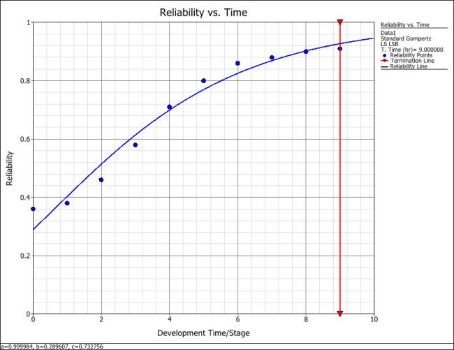
The standard Gompertz seems to do a fairly good job of modeling the data. However, it appears that it is having difficulty modeling the S-shape of the data. The modified Gompertz Reliability vs. Time plot is shown next. As expected, the modified Gompertz does a much better job of handling the S-shape presented by the data and provides a better fit for this data.
