How Good Is Your Assumed Distribution's Fit?

After fitting a distribution model to a data set when performing life data analysis, we are often interested in diagnosing the model's fit or comparing the fit of different distributions. In addition to the engineering knowledge that should always govern the choice of a distribution model, there are many statistical tools that can help in deciding whether or not a distribution model is a good choice from a statistical point of view. These tools can also be used to compare the fit of different distributions. This article presents a survey of various statistical tools available in Weibull++ that can be used to assess the fit of a distribution model and compare it to other distributions.

For the remainder of this article, we will use the following data set to explain the different ways to asses the fit of one or multiple distributions. For comparisons, we will use as an example the Weibull distribution and the exponential distribution. (Note, however, that the concept can be used to compare more than two distributions.)

Table 1: Sample data set

Failure Times
43
68
74
77
80
91
99
103
103
166

Probability Plots

Probability plotting is a graphical method that allows a visual assessment of the model fit. Once the model parameters have been estimated, the probability plot can be created. The next figure shows a comparison of the probability plots of two choices of distributions using the same data set.

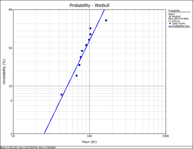
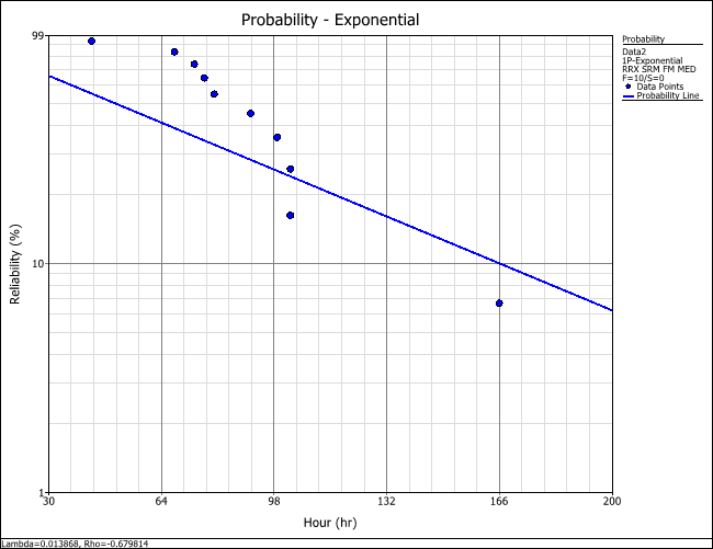
Figure 1: Comparing the probability plots of two distributions using the same data set

The plots show that the Weibull distribution fits the data well and is a better fit than the exponential distribution.

Note:
This method can be used if the Least Squares Parameter Estimation (Rank Regression) method has been used to estimate the parameters of the distribution. It should not be used if the MLE (Maximum Likelihood) parameter estimation method has been used to fit the distribution model. Even though it is common practice to plot the MLE solutions along with median ranks (i.e., points are plotted according to median ranks and the line according to the MLE solutions), this is not completely representative. The MLE method is actually independent of any kind of ranks. For this reason, the MLE solution often appears not to track the data on the probability plot. This is perfectly acceptable, as the two methods are independent of each other, and in no way suggests that the solution is wrong.

Correlation Coefficient

The correlation coefficient, usually denoted by ρ (Rho), is a measure of how well the linear regression model (the probability line) fits the data. In the case of life data analysis, it is a measure of the strength of the linear relation (correlation) between the median ranks and the data. The population correlation coefficient is defined as follows:

where σxy is the covariance of x (times-to-failure) and y (median ranks), σx is the standard deviation of x, and σy is the standard deviation of y.

The estimator of ρ is the sample correlation coefficient, $\hat{\rho}$ , given by:

MATH

The range of $\hat{\rho}$ is -1 ≤ $\hat{\rho}$ ≤ 1.

The closer the value of $\hat{\rho}$ is to 1 or -1 (or the closer the absolute value is to 1), the better the linear fit. Note that +1 indicates a perfect fit (i.e., the paired values (xi, yi) lie on a straight line) with a positive slope, while -1 indicates a perfect fit with a negative slope. A correlation coefficient value of zero would indicate that the data are randomly scattered and have no pattern or correlation in relation to the regression line model.

Using the data set presented in Table 1 and using the Rank Regression on X method to estimate the parameters, we make the following comparison:

Table 2: Comparing the correlation coefficients of two distributions using the same data set

Distribution Model	Weibull	Exponential
Parameters	β = 3.36, η = 100.05	λ = 0.0138
Correlation Coefficient, $\hat{\rho}$	0.95	-0.67

The above table shows that the Weibull distribution is a very adequate model (i.e., | $\hat{\rho}$ | is close to 1). Also, the absolute value of the correlation coefficient for the Weibull distribution is greater than that for the exponential distribution (i.e., the Weibull distribution is statistically a better fit).

Note:
The correlation coefficient value is displayed by default in Weibull++ below the estimated parameter values on the Main tab of the Standard Folio's Control Panel.

Likelihood Value

When using the MLE (Maximum Likelihood Estimation) method to estimate the parameters of the distribution model, the likelihood value can be used to assess the fit of the distribution to the data set. The likelihood value (or function), L, is the basis of the MLE parameter estimation method. It is mathematically formulated as follows:

MATH

where:

R is the number of units with exact times-to-failure.
M is the number of suspended units.
P is the number of units with left censored or interval times-to-failure.
θ1, θ2, ..., θk are the parameters of the distribution.
Ti is the ith time to failure.
Sj is the jth time of suspension.
$I_{l_{U}}$ is the ending of the time interval of the lth group.
$I_{l_{L}}$ is the beginning of the time interval of the lth group.

Unlike the correlation coefficient, the likelihood value is not constrained by a certain range of possible values. L can have any value and therefore cannot be used by itself to make a judgment about the fit of the distribution model. L can, however, be used to compare the fit of multiple distributions. The distribution with the largest L value is the best fit statistically.

Note that the likelihood values shown in Weibull++ are actually the log-likelihood values, not the likelihood values. The log-likelihood function is used instead because it is much easier to work with than L for parameter estimation. Using the log-likelihood function does not affect the validity of the results.

Using the data set presented in Table 1 and using the MLE method to estimate the parameters, we make the following comparison:

Table 3: Comparing the log-likelihood value of two distributions using the same data set

Distribution Model	Weibull	Exponential
Parameters	β = 3.03, η = 100.99	λ = 0.0111
Log-Likelihood Value	-48.42	-55.04

The above table shows that the log-likelihood value for the Weibull distribution is greater than that for the exponential distribution (i.e., the Weibull distribution is statistically a better fit).

Note:
The log-likelihood value is displayed by default in Weibull++ below the estimated parameter values on the Main tab of the Standard Folio's Control Panel.

Modified Kolmogorov-Smirnov (KS) Test

The standard Kolmogorov-Smirnov (KS) test can only be used when determining the fit of a continuous distribution with known parameters. In life data analysis, the parameters are typically unknown and need to be estimated from the sample data. Therefore, another type of KS test is used, called the Modified KS test.

If the data set is made of N failure times (t1, t2, ..., tN), we can define SN(t) to be the function giving the fraction of data points to the left of a given value ti(i = 1, 2,, ..., N). SN(t) is constant between consecutive tivalues, and jumps by the same constant 1/N value at each ti.

The Modified KS test uses Dmax, the maximum of the absolute difference between SN(t) and the fitted cumulative distribution function, Q(t). [Ref. 1]

What makes the Modified KS test useful is that its distribution in the case of the null hypothesis (i.e., data set drawn from the fitted distribution) can be calculated, at least to a useful approximation, thus giving the significance of any observed non-zero value of Dmax.

The Modified KS test returns the probability that DCRIT < Dmax. A high probability value, close to 1, indicates that there is a significant difference between the theoretical distribution and the data set.

Using the data set presented in Table 1 and using the MLE method to estimate the parameters, we make the following comparison:

Table 4: Comparing two distributions using the Modified Kolmogorov-Smirnov test

Distribution Model	Weibull	Exponential
Parameters	β = 3.03, η = 100.99	λ = 0.0111
*P(DCRIT < Dmax)*	14.84%	89.58%

The above figure shows that the value of P(DCRIT < Dmax) for the Weibull distribution is smaller than that for the exponential distribution (i.e., the Weibull distribution is statistically a better fit).

Note:

The Modified KS test can be used for small sample sizes.
The Modified KS test result can be obtained in Weibull++ by selecting Goodness of Fit Results from the Data menu.

Chi-Squared Test

The chi-squared test relies on the grouping (or binning) of the data into a number of intervals (as in histograms).

Suppose that Niis the number of data points in the ith bin and ni is the number expected according to the assumed distribution. The chi-squared statistic is then [Ref. 1]:

where the summation is over all bins. When the number of bins and the number of data points in each bin is sufficiently large (minimum sample size of 25-35 is recommended [Ref. 1]), it can be proved that the χ2 statistic follows a cumulative distribution that can be approximated by the chi-squared CDF. Notice that if the assumed distribution fit the data exactly, the χ2 statistic would be equal to zero. Therefore, a large value indicates a significant difference between the assumed distribution and the data set.

The chi-squared test returns a p-value, or the probability that a χ2 value larger than the observed value could occur provided that the data is well described by the assumed distribution. A small p-value indicates good agreement between the assumed distribution and the data set, while a p-value close to 1 indicates that there is a significant difference between the two.

Using the data set presented in Table 1 and using the MLE method to estimate the parameters, we make the following comparison:

Table 5: Comparing two distributions using the chi-squared test

Distribution Model	Weibull	Exponential
Parameters	β = 3.03, η = 100.99	λ = 0.0111
*p-value*	26.50%	66.76%

Table 5 shows that the p-value when the data are fitted with a Weibull distribution is smaller than that when the data are fitted with an exponential distribution (i.e., the Weibull distribution is statistically a better fit).

Note:

The chi-squared test is less powerful than the Modified KS test for any sample size. [Ref. 1]
The chi-squared test result can be obtained in Weibull++ by selecting Goodness of Fit Results from the Data menu.

References

1. Kececioglu, Dimitri, Reliability and Life Testing Handbook, Volume I, Prentice Hall, Inc., New Jersey, 1993.