Process Variation and Capability Assessment
Competitive companies understand that satisfying customers' needs and running a successful operation requires a system that is dependable, predictable and consistent. Many of today's quality management philosophies, such as Six Sigma, focus on reducing variations and scrap. A modern view of quality defines it as the inverse of variability. Therefore, measuring variability and finding ways to reduce it is important for the success of a company. This article presents a Weibull analysis approach to modeling production data for a process in order to assess its deviation and capabilities. This approach augments the Six Sigma-type calculations, which typically rely on the normality assumption.
We have discussed in past issues how process availability and throughput can be studied through the modeling of the process (for example, see Throughput Analysis (Part II)). This "in-depth" way of assessing a process yield can be complemented by a "higher view" approach that relies on using actual periodical production data of the system. This is a quick and useful way to assess the "health" of a process and it is a stepping stone for getting the process as close to the target as possible.
Introduction
Where does the "Sigma" in Six Sigma come from? Sigma is a statistical notation for the standard deviation parameter that can be used to quantify how far a given process deviates from perfection. The central idea behind Six Sigma is measuring the number of "defects" in a process and figuring out how to eliminate them in order to get the process more in line with its goal. "Defects" can be used in a more general context; the term could refer to any issues that cause concern to a company, such as defective products, out-of-specs products, inconsistency in production volumes, etc. Measuring defects also leads to discussions about the capability of the process to avoid defects, i.e. how far the process is from being the on-target, predictable and controlled process that the company hopes to have.
The next figure compares production volumes of two processes, a healthy one and a troubled one.
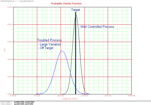
Figure 1 Two Different
Processes
In Six Sigma, variations are typically modeled with the bell-curve normal distribution. Oftentimes, processes and products are not "well-behaved" and their distributions are typically skewed. The skewness is generally more apparent when the variations are significant. Therefore, Six Sigma calculations have been criticized for relying heavily on the normality assumption.
In this article, we will focus on the Weibull distribution as our distribution model because of its flexibility and generally skewed pdf shape, as shown in Figure 2; however, other types of distributions (such as the lognormal, Gumbel and logistic distributions) might be appropriate depending on the types of variation.
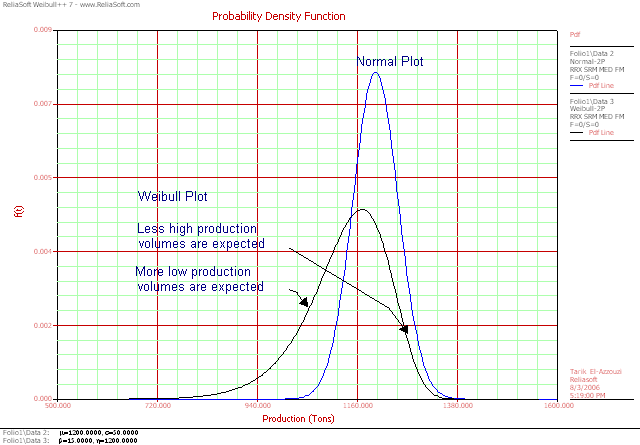
Figure 2 Normal and
Weibull pdf Plots Comparison
The following items are some of the key characteristics to look at when studying the probability plots of the process. These characteristics can help you discover signs of an unhealthy process.
-
Deviation from the target:
The next plot provides a good way to detect shift compared to an acceptable process that is centered. It also gives a visual idea of the production loss, inefficiencies and lost potential of the process.
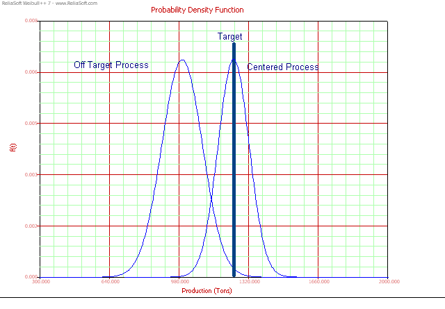
Figure 3 Process Showing
Significant Production Losses
-
Steepness of probability line or width of pdf:
This indicates the level of variation in the production. β is the slope parameter of the Weibull probability line. A small β value means a flatter probability line and wider pdf plot, all of which are signs of large variations and an unhealthy process. βs sister in the normal distribution is σ. In a process that follows a normal distribution, the smaller the σ, the better.
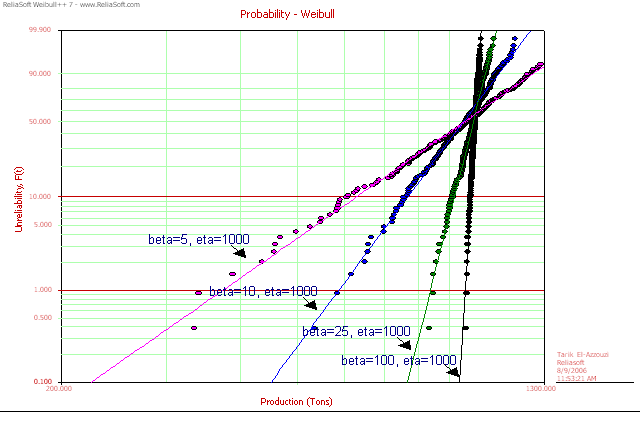
Figure 4 Probability Plot
for Processes with Different Variations Level
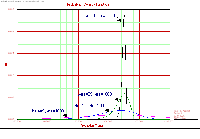
Figure 5 pdf Plot
for Processes with Different Variations Level
-
Signs of more causes of variation:
Look for curvature in the probability plot. This indicates that the production is not consistent in its variation and that there are different factors at work.
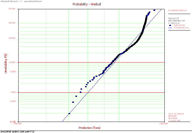
Figure 6 Process Showing
Mixed Variations Behavior
Such processes can be modeled with a mixed distribution such as the mixed Weibull distribution, which fits a set of Weibull distributions to subpopulations within the entire population and finds the percentage of each subpopulation. The same process shown in Figure 5 is modeled with a mixed Weibull distribution with two subpopulations; the probability plot is shown next.
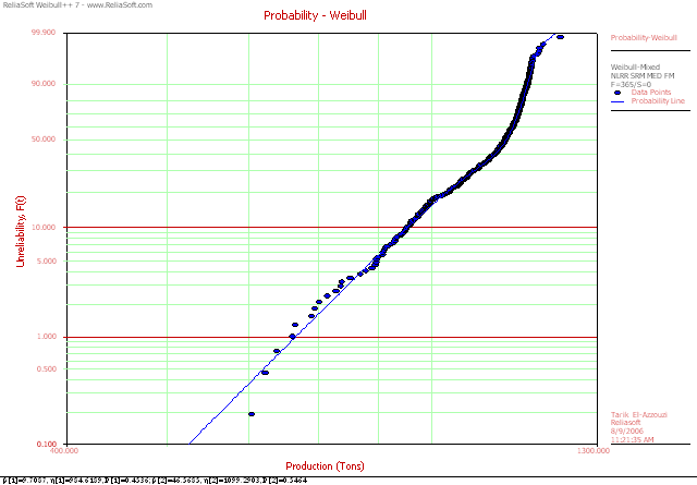
Figure 7 Process Showing
Mixed Variations Behavior Modeled with a Mixed Weibull Distribution
Example
A chemical manufacturer collected a sample from a years worth of production output logs. The manufacturers customer requires that the daily production volume should be at least 975 tons but no more than 1025 tons, in order to avoid unnecessary storage costs and deterioration problems. The data set is modeled in Weibull++.
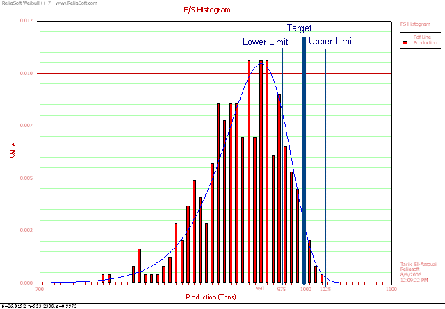
Figure 8 Process Sample
Production Data
The above graph shows that the process is off-target. It also does not follow the normal distribution, but rather a Weibull distribution with β=26.01. This indicates that the process suffers from significant variations.
Metrics such as Cp, Cpk and Cpm are common Six Sigma metrics used to assess the capabilities of a process. A great deal of importance is often assigned to these metrics, but they can be flawed because they assume that a process follows the normal distribution. Although some remedies have been suggested, such as using data transformation methods or modifying the way the process capability measures are calculated [1], these remedies remain unrobust and may complicate the analysis. We suggest using probability calculations, as they are straightforward and do not violate the assumptions of the chosen distribution. For this example, the percentage of daily productions that met the goal of 975 tons to 1025 tons can be found using the following probability calculations:
P(975<p<1025) = P(p<1025) P(p<975)
where p is a random variable that describes daily production. Calculating P(p<a) in Weibull++ means calculating the probability of failure by a. P(p<1025) and P(p<975) are found using Weibull++s QCP as follows.
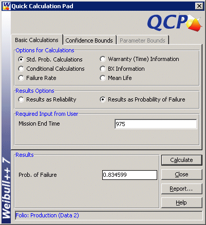
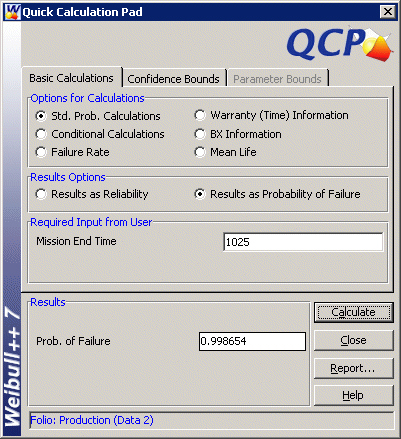
Therefore, P(975<p<1025) = P(p<1025) P(p<975) = 0.998654 0.834599 = 0.164055 or 16.4055%. In other words, 83.5945% of the days in the sample did not meet the production requirements.
It is important to convert your statistical analysis into money figures, which will have more impact on management and are more likely to motivate actions. Think about defects cost, scrapping cost, rework cost, penalties, lost revenue, customer dissatisfaction, etc. For this example, the manufacturer is penalized by its customer $1000 for every day of insufficient production and $500 for every day of excessive production that requires storage. For a one year period, the penalties amount to:
Penalties = 365.[P(p<975).$1000 + P(p>1025).$500]
Which is equivalent to:
Penalties = 365.[P(p<975).$1000 + (1-P(p<1025)).$500]
Therefore:
Penalties = 365.[0.834599.$1000 + (1-0.998654).$500]= $304,874.3
Conclusion
This article presented a Weibull analysis approach to model production data for a process. This is used to assess the variability in the process and discover a number of other types of signs of an "unhealthy" process. This approach does not rely on the questionable normality assumption in many Six Sigma calculations and provides an alternative to process capabilities calculations.
Reference
1. Montgomery, Douglas C., Introduction to Statistical Process Control, John Wiley & Sons, Inc., New York, pp. 444, 1997