Using the Fault Tree Method to Analyze Dependent and Independent Failure Modes

In Using Reliability Block Diagrams to Analyze Dependent and Independent Failure Modes, a method was presented for modeling dependent and independent failure modes using a reliability block diagram. In this article, we will revisit this topic. However, instead of using the reliability block diagram approach, the fault tree method will be incorporated utilizing BlockSim 6 FTI.

Example

Assume that a component can fail due to six independent primary failure modes: A, B, C, D, E and F. Some of these primary modes can be broken down further into the events that can cause them, or sub-modes. Furthermore, assume that once a mode occurs, the "event" also occurs and the mode does not go away. Specifically:

Component along with failure modes

The component fails if mode A, B or C occurs. If mode D, E or F occurs alone, the component does not fail; however, the component will fail if any two (or more) of these modes occur (i.e. D and E; D and F; E and F). Modes D, E and F have a constant rate of occurrence (exponential distribution) with mean times of occurrence of 200,000, 175,000 and 500,000 hours, respectively.

Objective

The objective of this example is to determine the following:

The reliability of the component after 1 year (8760 hrs).
The B10 life of the component.
The mean time to failure (MTTF) of the component.
Rank the modes in order of importance at 1 year.
Re-calculate results 1, 2 and 3 assuming mode B is eliminated.

To begin the analysis, modes A, B and C can be broken down further based on specific events (sub-modes), as defined next.

Mode A

There are five independent events (sub-modes) associated with mode A: events S1, S2, T1, T2 and Y. It is assumed that events S1 and S2 each have a constant rate of occurrence with a probability of occurrence of 1 in 10,000 and 1 in 20,000, respectively, in a single year (8760 hours). Events T1 and T2 are more likely to occur in an older component than a newer one (i.e. they have an increasing rate of occurrence) and have a probability of occurrence of 1 in 10,000 and 1 in 20,000, respectively, in a single year and 1 in 1,000 and 1 in 3,000, respectively, after two years. Event Y also has a constant rate of occurrence with a probability of occurrence of 1 in 1,000 in a single year. There are three possible ways for mode A to manifest itself:

Events S1 and S2 both occur.
Event T1 or T2 occurs.
Event Y and either event S1 or event S2 occur (i.e. events Y and S1 or events Y and S2).

The fault tree for mode A is shown in Figure 1.

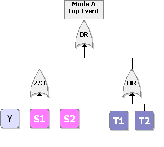
Figure 1: Fault tree for mode A

Each mode is identified as an event in the fault tree.

Mode A Discussion

The system reliability equation for this configuration (regardless of how it is drawn) is:

R(t)=-2R_T2R_S1R_S2R_T1R_Y+R_T2R_S1R_S2R_T1+R_T2R_S1R_T1R_Y+R_T2R_S2R_T1R_Y

The distribution parameters for each mode are computed in the same manner as previously discussed in Part I of this article.

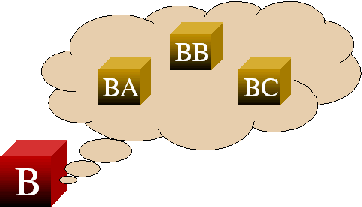
Mode B

The fault tree for mode B is shown in Figure 2.

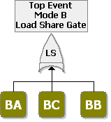
Figure 2: Fault tree for mode B (using a load sharing gate unique to BlockSim FTI)

Note that a "load sharing gate" is not a standard fault tree gate. BlockSim FTI introduces this gate to allow for representation of dependent events in a fault tree diagram. It behaves the same way as a load sharing container in an RBD.

Mode B Discussion

To describe the dependency, we need a model that describes how a life characteristic (in this case, the mean) changes as the events occur. Life-stress relationships used in accelerated testing provide a very good way to describe the effects of stress (load) on life. Since the failure rate is constant, the exponential distribution applies. Any standard life-stress relationship (i.e. an exponential curve or power curve) would apply equally because the function is only being evaluated at the two loads of interest and not necessarily extrapolating or interpolating between these two points. For simplicity, the Arrhenius life-stress relationship will be used.

Once the parameters have been obtained, the properties for each event for mode B are set. The load sharing container (if an RBD) or the gate (if a fault tree) properties for the events of mode B are shown in Figure 3.

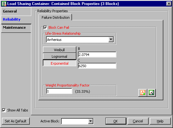
Figure 3: Arrhenius-exponential life-stress relationship properties

The reliability plot for this configuration is displayed in Figure 4.

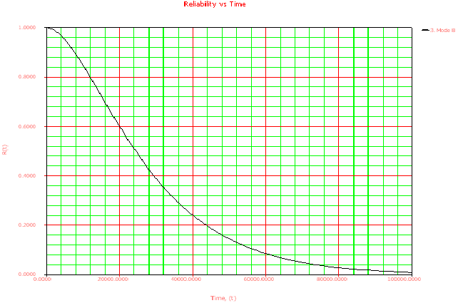
Figure 4: Reliability plot for mode B

For details on the exact reliability equation formulation, please refer to ReliaSoft's System Analysis Reference: Reliability, Availability and Optimization (the load sharing section).

Mode C

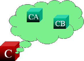
There are two sequential events associated with mode C: CA and CB. Both events must occur for mode C to occur. Event CB will only occur if event CA has occurred. If event CA has not occurred, then event CB will not occur. Both events CA and CB occur based on a Weibull distribution. For event CA, beta = 2 and eta = 30,000 hours. For event CB, beta = 2 and eta = 10,000 hours.

The fault tree for mode B is shown in Figure 5.

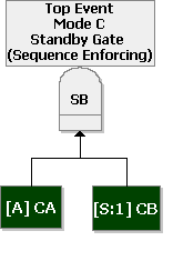
Figure 5: Sequence enforcing (standby) gate for mode C

Mode C Discussion

The failure distribution settings for event CA are shown in Figure 6.

Figure 6: Failure distribution settings for event CA

The failure distribution properties for event CB are set in the same manner.

Modes D, E and F

Modes D, E and F can all be represented using the exponential distribution. The failure distribution properties for modes D, E and F are presented next.

D: MTTF = 200,000 hours
E: MTTF = 175,000 hours
F: MTTF = 500,000 hours

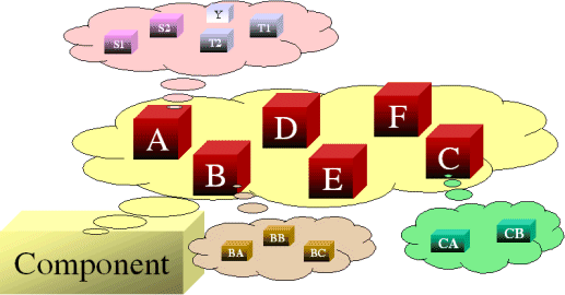
Component

The last step is to set up the component based on the primary modes (A, B, C, D, E and F). Modes A, B and C can each be represented by single blocks that encapsulate the subdiagrams already created. The fault tree in Figure 7 represents the primary failure modes for the component.

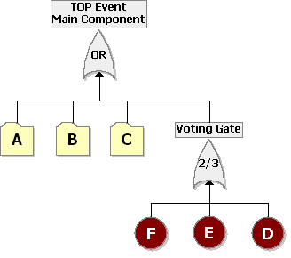
Figure 7: Fault tree of component

The voting gate in the fault tree accomplishes a 2-out-of-3 configuration. Subdiagrams are used for the sub-modes. Once the diagrams have been created, the reliability equation for the system can be obtained, as follows:

R(t)_System =R_AR_BR_FR_DR_C+R_AR_BR_FR_CR_E+R_AR_BR_DR_CR_E-2(R_AR_BR_FR_DR_CR_E)

Where R_A, R_B and R_Care the reliability equations corresponding to the sub-modes.

Analysis

The answers to the questions posed earlier can be answered using BlockSim 6. Regardless of the approach used (i.e. RBD or fault tree), the answers are the same.

The reliability of the component at 1 year (8760 hours) can be calculated using the Analytical Quick Calculation Pad (QCP) or by viewing the reliability vs. time plot, as displayed in Figure 8.

Figure 8: Reliability vs. time plot for component

Therefore, R(t = 8760) = 86.4975%.

Using the Analytical QCP, the B10 life of the component is equal to 7,373.94 hours.
Using the Analytical QCP, the mean life of the component is equal to 21,659.68 hours.
The ranking of the modes after 1 year can be shown via the static reliability importance plot, as shown in Figure 9.

Figure 9: Static reliability importance for each of the modes at t = 8,760 hours

Re-computing the results for 1, 2 and 3 assuming mode B is removed:

R = 98.72%

B10 = 16,928.38 hours

MTTF = 34,552.89 hours

Discussion

There are many options for modeling systems with fault trees and RBDs in BlockSim FTI. The following figures illustrate some of these options.

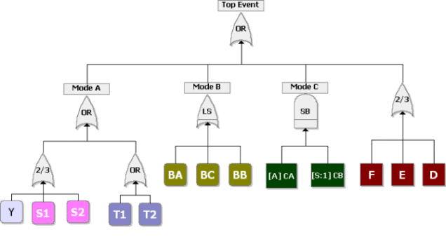
Figure 10: Fault tree of Figure 7 without using subdiagrams (transfers)

The component can be represented by an RBD, as shown in Part I of this article. Expanding on this concept, you can represent the component using an RBD where the subdiagrams are fault trees, as shown in Figure 11.

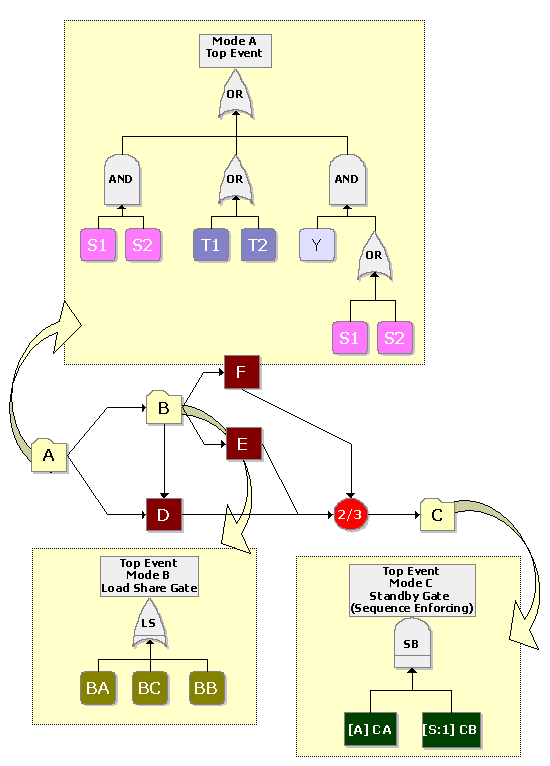
Figure 11: RBD of component using fault trees as subdiagrams

Now, using the same idea, the fault tree can contain transfers that link to reliability block diagrams, as shown in Figure 12.

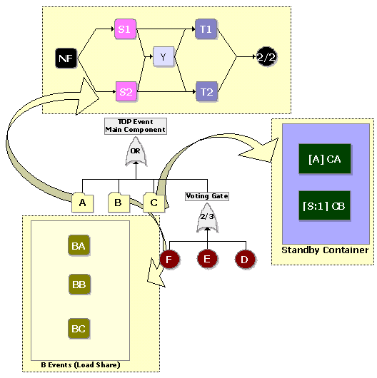
Figure 12: Fault tree of component using RBDs as subdiagrams