Using Reliability Block Diagrams to Analyze Dependent and Independent Failure Modes

When thinking of a reliability block diagram (RBD), the application that most often comes to mind is the analysis of a system based on the component reliabilities. You can also use the same methodology for a single component and its associated failure modes. In analyzing this scenario, both independent (i.e., if one mode occurs, the rest are not more likely to occur) and dependent modes (i.e., if one mode occurs, the rest are more likely to occur) can be included. To illustrate this, a component with multiple primary modes as well as multiple secondary modes (sub-modes) will be considered. In addition, both independence and dependence will be utilized.

Example

Assume that a component can fail due to six independent primary failure modes: A, B, C, D, E and F. Some of these primary modes can be broken down further into the events that can cause them, or sub-modes. Furthermore, assume that once a mode occurs, the "event" also occurs and the mode does not go away. (The aspect of a self-correcting mode will be discussed in an upcoming Hotwire article.) Specifically:

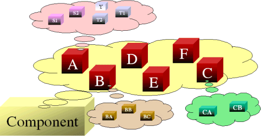
The component fails if mode A, B or C occurs. If mode D, E or F occurs alone, the Component does not fail; however, the Component will fail if any two (or more) of these modes occur (i.e. D and E; D and F; E and F). Modes D, E and F have constant rates of occurrence (exponential distribution) with mean times of occurrence of 200,000, 175,000 and 500,000 hours, respectively.

Objective

The objective of this example is to determine the following:

1. The reliability of the component after 1 year (8760 hrs).

2. The B10 life of the component.

3. The mean-time-to-failure of the component

4. Rank the modes in order of importance at 1 year.

5. Re-calculate Steps 1, 2 and 3 assuming that mode B is eliminated.

To begin the analysis, modes A, B and C can be broken down further based on specific events occurring (sub-modes), as defined next.

Mode A

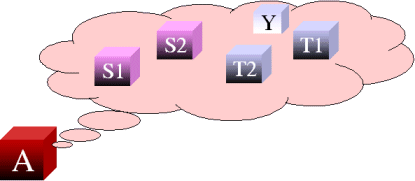
There are five independent events (sub-modes) associated with mode A: events S1, S2, T1, T2 and Y. It is assumed that events S1 and S2 each have a constant rate of occurrence with a probability of occurrence of 1 in 10,000 and 1 in 20,000, respectively, in a single year (8760 hours). Events T1 and T2 are more likely to occur in an older component than a newer product (i.e. they have an increasing rate of occurrence) and have a probability of occurrence of 1 in 10,000 and 1 in 20,000, respectively, in a single year and 1 in 1,000 and 1 in 3,000, respectively, after two years. Event Y also has a constant rate of occurrence with a probability of occurrence of 1 in 1,000 in a single year. There are three possible ways for mode A to manifest itself:

• Events S1 and S2 both occur.
• Event T1 or T2 occurs.
• Event Y and either event S1 or event S2 occur (i.e. events Y and S1 or events Y and S2).

The RBD that satisfies the conditions for mode A is shown in Figure 1.

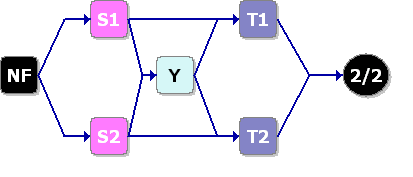
Figure 1: Reliability block diagram for mode A

The system reliability equation for this configuration is:

R(t)=-2R_T2R_S1R_S2R_T1R_Y+R_T2R_S1R_S2R_T1+R_T2R_S1R_T1R_Y+R_T2R_S2R_T1R_Y

Each mode is identified in the RBD. Furthermore, two additional items are included: a starting block (NF) and an end node (2/2). The starting block and the end node are set so they cannot fail and, therefore, will not affect the results. The end node is used to define a 2-out-of-2 k-out-of n configuration (i.e., both paths leading into the node must work).

Based on the given probabilities, distribution parameters can be computed for each block. For events S1, S2 and Y, an exponential distribution can be utilized because a constant rate was assumed. For event S1, the probability is 1 in 10,000 in one year (8760 hours). Therefore:

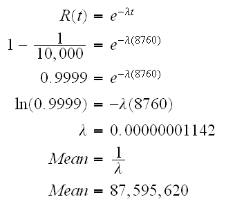
This could also be repeated using the Parameter Experimenter in BlockSim 7, as shown in Figure 2.

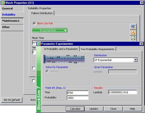
Figure 2: BlockSim's Parameter Experimenter

The mean for events S2 and Y can be computed in a similar manner. Events T1 and T2 need to be modeled using a life distribution that does not have a constant failure rate. Using BlockSim's Parameter Experimenter and selecting the Weibull distribution, the parameter values for events T1 and T2 are shown in Figures 3 and 4, respectively.

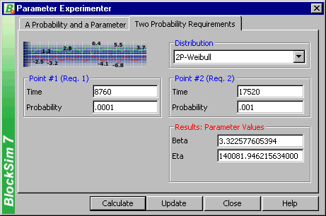
Figure 3: Parameter values for event T1

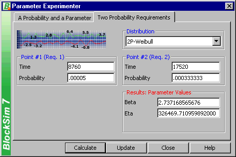
Figure 4: Parameter values for event T2

Mode B

There are three dependent events associated with mode B: events BA, BB and BC. Two out of the three events must occur for mode B to occur. Events BA, BB and BC have an exponential distribution with a mean of 50,000 hrs. The events are dependent (i.e. if BA, BB or BC occurs, the remaining events are more likely to occur). Specifically, when one event occurs, the MTTF of the remaining events is cut in half. This is basically a load sharing configuration. The reliability function for each block will change depending on the other events. Therefore, the reliability of each block is not only dependent on time, but also on the stress (load) that the block sees.

The representative reliability block diagram for mode B is shown in Figure 5.

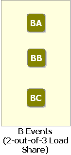
Figure 5: Reliability block diagram for mode B

To describe the dependency, we need a model that describes how a life characteristic (in this case, the mean) changes as the events occur. Life-stress relationships used in accelerated testing provide a very good way to describe the effects of stress (load) on life. Since the failure rate is constant, the exponential distribution applies. Any standard life-stress relationship (i.e. an exponential curve or power curve) would apply equally because the function is only being evaluated at the two loads of interest and not necessarily extrapolating or interpolating between these two points. For simplicity, the Arrhenius life-stress relationship will be used.

The exponential pdf is given by:

And its mean is equal to:

Therefore:

The Arrhenius-exponential pdf can then be obtained by setting:

The Arrhenius-exponential pdf is then represented by the following:

Once the life-stress relationship has been established, we need to define the stresses (loads).  Based on the problem statement, we can say that when all three blocks representing events BA, BB and BC are working, the load is 1. When one fails, the other two must take on the load of the failed unit, thus they take on an additional 50% of the total load. The model parameters can easily be computed from ALTA 7, as shown in Figure 6.

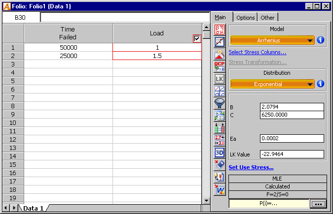
Figure 6: Parameter values using ALTA 7

Alternatively, the Load & Life Parameter Experimenter in BlockSim can also be used, as shown in Figure 7.

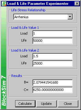
Figure 7: Load & Life Parameter Experimenter in BlockSim 7

Once the parameters have been obtained, the properties for each event for mode B are set. The load sharing container properties for the events of mode B are shown in Figure 8.

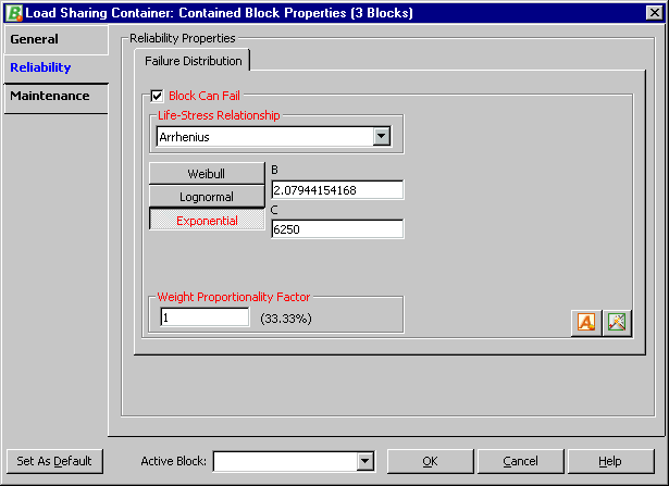
Figure 8: Arrhenius-exponential life-stress relationship properties

The reliability plot for this configuration is displayed in Figure 9.

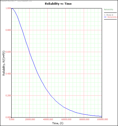
Figure 9: Reliability plot for mode B

For details on the exact reliability equation formulation, please refer to ReliaSoft's System Analysis Reference: Reliability, Availability and Optimization.

Mode C

There are two sequential events associated with mode C: CA and CB. Both events must occur for mode C to occur. Event CB will only occur if event CA has occurred. If event CA has not occurred, then event CB will not occur. Both events CA and CB occur based on a Weibull distribution. For event CA, beta = 2 and eta = 30,000 hours. For event CB, beta = 2 and eta = 10,000 hours.

To model this, you can think of a scenario similar to standby redundancy. Basically, if CA occurs then CB gets initiated. A standby container can be used to model this, as shown in Figure 10.

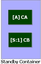
Figure 10: Standby container for mode C 

In this case, event CA is set as the active component and CB as the standby. If event CA occurs, CB will be initiated. For this analysis, a perfect switch is assumed. The properties are set in BlockSim as follows:

• Contained Items

  • CA: Active failure distribution, Weibull distribution (beta = 2, eta = 30,000).

  • CA: Quiescent failure distribution: None, cannot fail or age in this mode.

  • CB: Active failure distribution, Weibull distribution (beta = 2, eta = 10,000).

  • CB: Quiescent failure distribution: None, cannot fail or age in this mode.

• Switch

  • Active Switching: Always works (100% reliability) and instant switch (no delays).

  • Quiescent Switch failure distribution: None, cannot fail or age in this mode.

The failure distribution settings for event CA are shown in Figure 11.

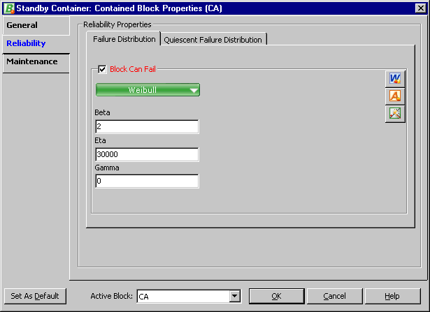
Figure 11: Failure distribution settings for event CA

The failure distribution properties for event CB are set in the same manner.

Modes D, E and F

Modes D, E and F can all be represented using the exponential distribution. The failure distribution properties for modes D, E and F are presented next.

• D: MTTF = 200,000 hours

• E: MTTF = 175,000 hours

• F: MTTF = 500,000 hours

Component

The last step is to set up the component based on the primary modes (A, B, C, D, E and F). Modes A, B and C can each be represented by single blocks that encapsulate the subdiagrams already created.  The RBD in Figure 12 represents the primary failure modes for the component.

 

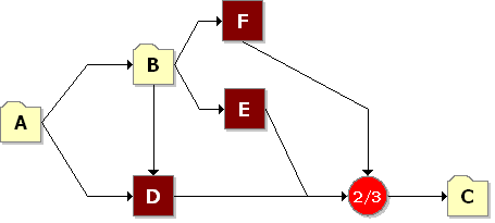
Figure 12: RBD of Component

The node represented by 2/3 indicates a 2-out-of-3 configuration. Once the diagram has been created, the reliability equation for the system can be obtained, as follows:

R(t)_System =R_AR_BR_FR_DR_C+R_AR_BR_FR_CR_E+R_AR_BR_DR_CR_E-2(R_AR_BR_FR_DR_CR_E)

Where R_A, R_B and R_C are the reliability equations corresponding to the sub-modes.

Analysis

The answers to the questions posed earlier can be answered using BlockSim.

1) The reliability of the component at 1 year (8760 hours) can be calculated using the Analytical Quick Calculation Pad (QCP) or by viewing the reliability vs. time plot, as displayed in Figure 13.

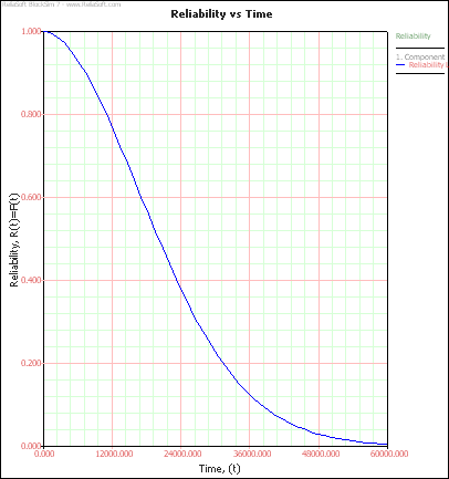
Figure 13: Reliability vs. time plot for component

Therefore, R(t = 8760) = 86.4978%.

2) Using the Analytical QCP, the B10 life of the component is equal to 7,373.94 hours.

3) Using the Analytical QCP, the mean life of the component is equal to 21,664.02 hours.

4) The ranking of the modes after 1 year can be shown via the static reliability importance plot, as shown in Figure 14.

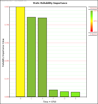
Figure 14: Static reliability importance for each of the modes at t = 8760 hours

5) Re-computing the results for 1, 2 and 3 assuming mode B is removed:

• R = 98.72%

• B10 = 16,928.38 hours

• MTTF = 34,552.89 hours

Previous articles that also discuss load sharing include: "Determining the Reliability of a System with Load Sharing," "Updating the Classic Reliability Block Diagram Methodology and Constructs" and "Using QALT Models to Analyze System Configurations with Load Sharing."

Previous articles that also discuss standby redundancy include: "Determining the Reliability of a System with Standby Redundancy," "Reliability of Standby Systems with a Switching Device" and "Updating the Classic Reliability Block Diagram Methodology and Constructs."