Improving Product Reliability Using Design of Experiments

Design of Experiments (DOE) has been widely used to quickly identify important factors and to determine the best values of them in order to optimize the performance of a product or process. In this article, we will give an example using DOE++ to improve product reliability, and at the same time make sure the product meets its functional requirement.

Problem Statement:

After conducting a fractional factorial design, engineers identified the following three factors as important design and manufacturing variables that affect the output volume of a device.

• Thickness (range from 2 - 6 inches)
• Tuning time (range from 10 - 50 minutes)
• Width (range from 8 - 18 inches)

To meet the design specification, the volume of this device must be around 80 gallons per hour. The acceptable range is from 75 to 85 gallons per hour. It was also noticed that changing the above three factors will affect the reliability of the device. Therefore, we need to find the settings of these three factors that will meet the volume requirement, but at the same time will not reduce the reliability too much.

Design the Experiment:

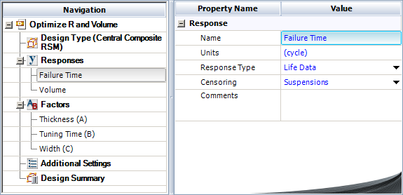
1. Responses: The responses in the study are volume and cycles to failure. In the test, we need to record the average volume and cycles to failure of each test unit. Note that we configure the Failure Time response as suspended life data, as shown next.



2. Factors: The factors are the three factors given above. The following values are used to define the high and the low value for each factor:
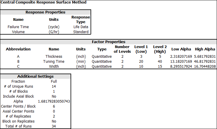
   • Thickness (Low = 3, High = 5 inches)
   • Tuning time (Low = 20, High = 40 minutes)
   • Width (Low = 10, High = 15 inches)
3. Design an Experiment: Since the objective of the study is to optimize the output volume of the device, we use a central composite design. Central composite design is one design type of the response surface method (RSM), and is very efficient for optimization. We also decide to use two replicates and six center points in this study.
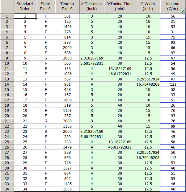
4. Conduct the Test: The test lasts for 2,000 cycles and we record the failure time and volume information of each test sample. If a test sample is still working by the end of the test, then we use 2,000 cycles as the censoring time for this sample.

The experiment design is summarized below.



5. Collect Test Results: The data set is given below.

Analyze the Data

The statistical method used for analyzing the response of volume is different from the method used for the cycles to failure.

For volume, the regression model is:

(1)

where:

• yi is the volume per hour of the ith test sample.
• x1i is the value of factor A (thickness) of the ith test sample.
• x2i is the value of factor B (tuning time) of the ith test sample.
• x3i is the value of factor C (width) of the ith test sample.
• εi is the error term.

The ANOVA table is given below.

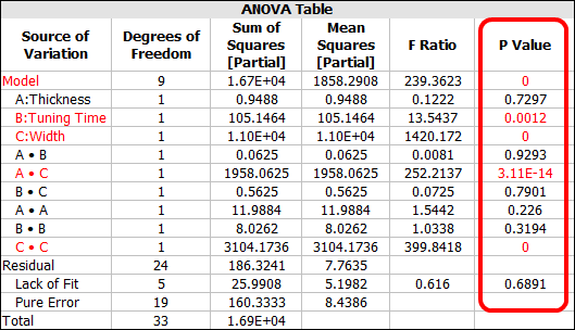
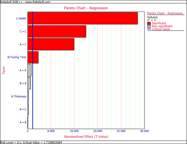
The P Value column shows that B, C, AC and CC are significant terms. B and C are the linear effect of tuning time and width. AC is the interaction effect of the thickness and width. CC represents the quadratic effect of the width. The results also can be seen from the Regression plot:

To reduce the prediction uncertainty, we removed the insignificant terms from the model so that we could use only the significant terms in the final model for the volume, then reanalyzed the data. The final model is shown next:

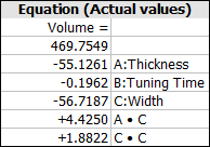
Therefore, the linear regression equation is:

For the failure response, since we have suspensions, and the suspension times are not "cycles to failure," we cannot use the regular regression model. Instead, we need to assume that the cycles to failure follow a certain distribution and the life characteristic of the distribution is affected by the factor values. In this example we use the Weibull distribution where its life characteristic is the scale parameter η. Since η must be a positive value, it uses the following regression equation:

(2)

where ηi represents the life for the ith observation. The life of the ith observation follows a Weibull distribution with the parameters being β and ηi. The probability density function of this Weibull distribution is:

(3)

For more discussion on the theory of lifetime modeling, please refer to the Life Data Analysis Reference Book and the "Reliability DOE for Life Tests" chapter of the Experiment Design and Analysis Reference.

We use the likelihood ratio test to test the significance of each term in the model and the results are given below:

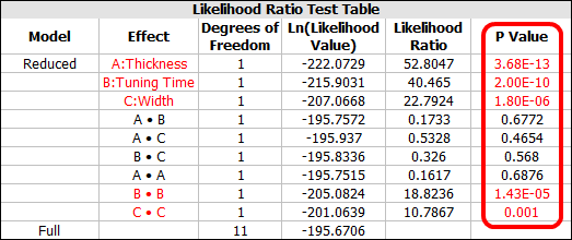
The P Value column shows that A, B, C, BB and CC are significant. The results also can be seen from the Regression plot:

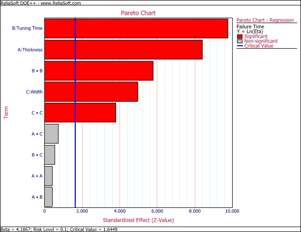
By removing the non-significant terms and recalculating the results, we obtain the final regression model as:

As shown in the following table, the calculated beta for the Weibull distribution is 4.1168.

Optimization

Once we have obtained the final model for each response, we can use them to find the suitable value for each factor that can meet the volume and reliability requirement.

The reliability is required to be at least 95% at 2,000 hours. Based on this requirement, we can calculate the required value for η in the Weibull distribution. Using the Quick Parameter Estimator, we get:

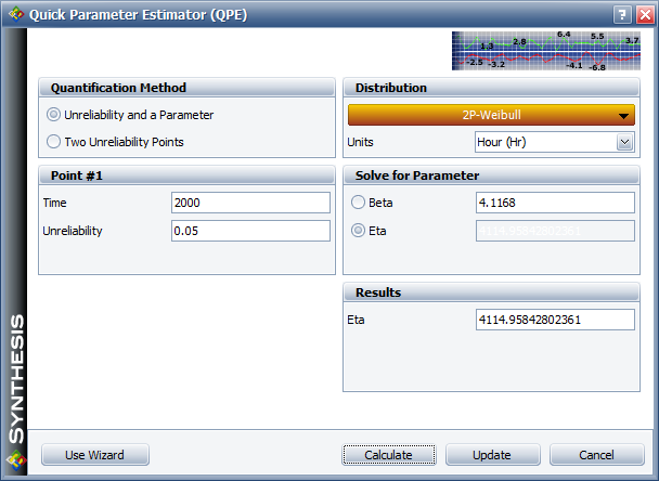
The calculated η is 4,114.96. Therefore, ln(η) must be greater than ln(4114.96) = 8.3224. We then use this information as the requirement for the lower limit in the optimization settings.

For volume, we know its target value is 80 and should be within the range of 75 to 85. Therefore, the optimization settings are:

The optimization result is:

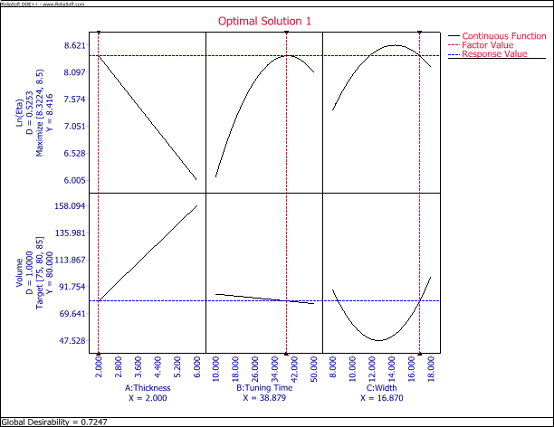
The above result shows that the best settings for these three factors are:

• Thickness = 2 inches.
• Tuning time = 38.879 minutes (which can be rounded to 39 minutes).
• Width = 16.87 inches (which can be rounded to 17 inches).

We can create a custom solution using the rounded values as these will make the manufacturing process easier.

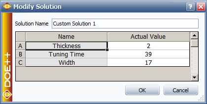
The predicted volume and ln(η) with these settings are:

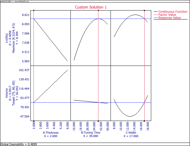
From the plot we can see that the predicted volume is 82.042 gallons per hour and the ln(η) is 8.394. Both results still can meet the requirement.

With these settings, the predicted η is 4,420 and the corresponding reliability at 2,000 hours is 0.9625.

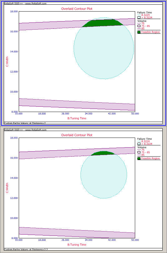
In fact, there are multiple settings of these three factors that can meet the requirement. The optimization plot only gives the best one. We can view these settings from the contour plot using the following settings:

The green area on a plot is the feasible region where both the volume and reliability requirement can be met. We generate the following plots by setting X as tuning time, Y as width, and an increasing thickness from 2 to 6 with a certain increment.

Conclusion

In this article, we presented an example of how to use Design of Experiments to optimize reliability and other performance factors. When conducting product prototype tests, there are usually many performance responses that are affected by many inputs such as design parameters and process variables. In order to make all the responses meet their requirements, multiple response optimization should be used. Design of Experiments provides an efficient way to identify important factors and find the best settings of these factors.