Life Data Analysis (Weibull Analysis)

An Overview of Basic Concepts

In life data analysis (also called "Weibull analysis"), the practitioner attempts to make predictions about the life of all products in the population by fitting a statistical distribution to life data from a representative sample of units. The parameterized distribution for the data set can then be used to estimate important life characteristics of the product such as reliability or probability of failure at a specific time, the mean life and the failure rate. Life data analysis requires the practitioner to:

• Gather life data for the product.
• Select a lifetime distribution that will fit the data and model the life of the product.
• Estimate the parameters that will fit the distribution to the data.
• Generate plots and results that estimate the life characteristics of the product, such as the reliability or mean life.

This document presents an overview of basic concepts in life data analysis (Weibull analysis) and some suggestions for additional research. ReliaSoft's Weibull++ software provides a complete array of life data analysis tools.

Life Data

The term "life data" refers to measurements of product life. Product life can be measured in hours, miles, cycles or any other metric that applies to the period of successful operation of a particular product. Since time is a common measure of life, life data points are often called "times-to-failure" and product life will be described in terms of time throughout the rest of this guide. There are different types of life data and because each type provides different information about the life of the product, the analysis method will vary depending on the data type. With "complete data," the exact time-to-failure for the unit is known (e.g., the unit failed at 100 hours of operation). With "suspended" or "right censored" data, the unit operated successfully for a known period of time and then continued (or could have continued) to operate for an additional unknown period of time (e.g., the unit was still operating at 100 hours of operation). With "interval" and "left censored" data, the exact time-to-failure is unknown but it falls within a known time range. For example, the unit failed between 100 hours and 150 hours (interval censored) or between 0 hours and 100 hours (left censored).

Lifetime Distributions (Life Data Models)

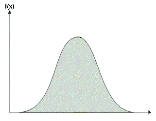
Statistical distributions have been formulated by statisticians, mathematicians and engineers to mathematically model or represent certain behavior. The probability density function (pdf) is a mathematical function that describes the distribution. The pdf can be represented mathematically or on a plot where the x-axis represents time, as shown next. 

The equation below gives the pdf for the 3-parameter Weibull distribution. Some distributions, such as the Weibull and lognormal, tend to better represent life data and are commonly called "lifetime distributions" or "life distributions." In fact, life data analysis is sometimes called "Weibull analysis" because the Weibull distribution, formulated by Professor Waloddi Weibull, is a popular distribution for analyzing life data. The Weibull model can be applied in a variety of forms (including 1-parameter, 2-parameter, 3-parameter or mixed Weibull). Other commonly used life distributions include the exponential, lognormal and normal distributions. The analyst chooses the life distribution that is most appropriate to model each particular data set based on past experience and goodness-of-fit tests.

Parameter Estimation

In order to fit a statistical model to a life data set, the analyst estimates the parameters of the life distribution that will make the function most closely fit the data. The parameters control the scale, shape and location of the pdf function. For example, in the 3-parameter Weibull model (shown above), the scale parameter, η, defines where the bulk of the distribution lies. The shape parameter, β, defines the shape of the distribution and the location parameter, γ, defines the location of the distribution in time. [View a visual demonstration of the effect of the parameters on the probability density function...]

Several methods have been devised to estimate the parameters that will fit a lifetime distribution to a particular data set. Some available parameter estimation methods include probability plotting, rank regression on x (RRX), rank regression on y (RRY) and maximum likelihood estimation (MLE). The appropriate analysis method will vary depending on the data set and, in some cases, on the life distribution selected.

Calculated Results and Plots

Once you have calculated the parameters to fit a life distribution to a particular data set, you can obtain a variety of plots and calculated results from the analysis, including:

• Reliability Given Time: The probability that a unit will operate successfully at a particular point in time. For example, there is an 88% chance that the product will operate successfully after 3 years of operation.
• Probability of Failure Given Time: The probability that a unit will be failed at a particular point in time. Probability of failure is also known as "unreliability" and it is the reciprocal of the reliability. For example, there is a 12% chance that the unit will be failed after 3 years of operation (probability of failure or unreliability) and an 88% chance that it will operate successfully (reliability). 
• Mean Life: The average time that the units in the population are expected to operate before failure. This metric is often referred to as "mean time to failure" (MTTF) or "mean time before failure" (MTBF). 
• Failure Rate: The number of failures per unit time that can be expected to occur for the product.
• Reliable Life (warranty time). The estimated time when the reliability will be equal to a specified goal. For example, the estimated time of operation is 4 years for a reliability of 90%.
• B(X) Life: The estimated time when the probability of failure will reach a specified point (X%). For example, if 10% of the products are expected to fail by 4 years of operation, then the B(10) life is 4 years. (Note that this is equivalent to a reliable life of 4 years for a 90% reliability.)
• Probability Plot: A plot of the probability of failure over time. (Note that probability plots are based on the linearization of a specific distribution. Consequently, the form of a probability plot for one distribution will be different than the form for another. For example, an exponential distribution probability plot has different axes than those of a normal distribution probability plot.)
• Reliability vs. Time Plot: A plot of the reliability over time.
• pdf Plot: A plot of the probability density function (pdf).
• Failure Rate vs. Time Plot: A plot of the failure rate over time.
• Contour Plot: A graphical representation of the possible solutions to the likelihood ratio equation. This is employed to make comparisons between two different data sets.

Confidence Bounds

Because life data analysis results are estimates based on the observed lifetimes of a sampling of units, there is uncertainty in the results due to the limited sample sizes. "Confidence bounds" (also called "confidence intervals") are used to quantify this uncertainty due to sampling error by expressing the confidence that a specific interval contains the quantity of interest. Whether or not a specific interval contains the quantity of interest is unknown.

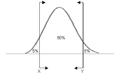
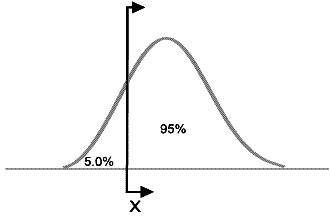
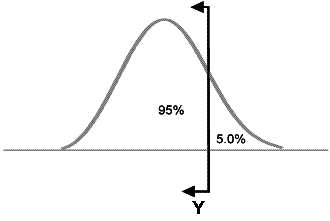
Confidence bounds can be expressed as two-sided or one-sided. Two-sided bounds are used to indicate that the quantity of interest is contained within the bounds with a specific confidence. One-sided bounds are used to indicate that the quantity of interest is above the lower bound or below the upper bound with a specific confidence. The appropriate type of bounds depends on the application. For example, the analyst would use a one-sided lower bound on reliability, a one-sided upper bound for percent failing under warranty and two-sided bounds on the parameters of the distribution. (Note that one-sided and two-sided bounds are related. For example, the 90% lower two-sided bound is the 95% lower one-sided bound and the 90% upper two-sided bounds is the 95% upper one-sided bound.)

Two-Sided Confidence Bounds
Lower One-Sided Confidence Bounds	Upper One-Sided Confidence Bounds