Warranty Analysis
Development testing allows you to uncover and correct reliability problems before a product is deployed; however, there are instances when a problem is not discovered until the product is in the customer’s hands. Data obtained from field failures can provide valuable information about how a product actually performs in the real world. Further, this life distribution is more reflective of failures that happen in the field under real use conditions and can be invaluable in planning developmental tests of new, similar designs.
In this example, you will extract life data from warranty returns records, and then compare the results obtained from the field data to the results obtained from an in-house reliability test.
In this scenario, we compared two bulbs for our new projector design, bulbs A and B. We recommended bulb A because of its higher reliability; however, bulb B is lower-priced, and so a decision was reached by management to use bulb B for production. The projectors with bulb B were then released to market with a 12-month warranty.
Soon after the product introduction, due to excessive returns (as you predicted), management decided to discontinue the use of bulb B and return to bulb A, which you originally recommended. Specifically, bulb B was used in production for twelve months. After that, any projectors released in the 13th month and beyond were modified to use bulb A. Six months after this change, you are asked to forecast the warranty returns due to bulb failures for the next six months. The returns data are available and shown in the following table. The data set is organized in Nevada chart format and it includes all 18 months of service (12 with bulb B and 6 with bulb A).
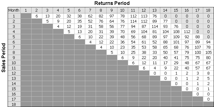
In this format, the columns represent the warranty returns periods and the rows represent the sales periods. This chart indicates, for example, that a total of 18 units were returned during the 3rd month (column 3), and that 13 of those units were sold in the first month (row 1) while 5 units were sold in the 2nd month (row 2). The rest of the chart can be read in a similar manner.
Objectives
- Assuming an average sales of 1,000 projectors per month, estimate the number of warranty returns due to bulb failures that will occur in the next six months (i.e., months 19 to 24).
- Optionally, verify whether an assumption of a usage rate of 50 hours/month per projector holds true for bulb B. This can be done by comparing warranty returns to a life data folio containing the following test data for bulb B:
|
State (F/S) |
Time (hrs) |
|
F |
300 |
|
F |
440 |
|
F |
495 |
|
S |
500 |
|
S |
500 |
Solution
You create a warranty analysis folio by choosing Home > Insert > Warranty.
![]()
When prompted to specify the data format, you select I want to enter data in the Nevada chart format, and then click Next.
Currently, there are 18 sales periods (i.e., the projectors with bulb B were sold in the first 12 months and the projectors with bulb A were sold in the following 6 months) and 18 returns periods. You are asked to forecast the returns for the next 6 months, so you include the forecasted future sales for the next 6 months. Note that because all new projectors have bulb A in them, the future sales will be of projectors with this type of bulb. You set up your Nevada chart with the following settings:

Note: In the Warranty Folio Setup window, you could select to label the periods in terms of months instead of numbers; however, the setup will require you to specify the calendar year. This example does not analyze several years of data, so we will simplify the data entry process by labeling the periods in terms of numbers instead of months.
(You’ll notice that in the screenshots here, we’ve called this folio "Warranty - Bulbs." If you want to rename your new folio, right-click the name in the current project explorer and choose Rename.)
When the folio has been created, you click the Change Units icon on the control panel.
![]()
You then specify that the time units of the sales and returns periods will be in terms of months.
Next, you enter data in the Sales data sheet. You use the assumption of a constant rate of sales of 1,000 projectors per month, and use the subset ID column to specify the type of bulb that was used in the projectors that were sold that month.
Note: Subset IDs allow you to separate the full data into different homogeneous data sets. In this example, there are two products, bulb A and bulb B. Separating the data by product will allow you to fit different models (distribution and parameters) to each one.
The resulting Sales data sheet is shown next.

| Quantity In-Service | Subset ID |
| 1000 | Bulb B |
| 1000 | Bulb B |
| 1000 | Bulb B |
| 1000 | Bulb B |
| 1000 | Bulb B |
| 1000 | Bulb B |
| 1000 | Bulb B |
| 1000 | Bulb B |
| 1000 | Bulb B |
| 1000 | Bulb B |
| 1000 | Bulb B |
| 1000 | Bulb B |
| 1000 | Bulb A |
| 1000 | Bulb A |
| 1000 | Bulb A |
| 1000 | Bulb A |
| 1000 | Bulb A |
| 1000 | Bulb A |
| 1000 | Bulb A |
| 1000 | Bulb A |
| 1000 | Bulb A |
| 1000 | Bulb A |
| 1000 | Bulb A |
| 1000 | Bulb A |
You then enter the data from the Nevada chart given earlier to the Returns data sheet of the folio.
| 1 | 2 | 3 | 4 | 5 | 6 | 7 | 8 | 9 | 10 | 11 | 12 | 13 | 14 | 15 | 16 | 17 | 18 |
| 6 | 13 | 20 | 32 | 38 | 62 | 82 | 97 | 78 | 112 | 113 | 76 | 0 | 0 | 0 | 0 | 0 | |
| 5 | 9 | 20 | 35 | 52 | 76 | 64 | 76 | 114 | 112 | 89 | 77 | 0 | 0 | 0 | 0 | ||
| 4 | 12 | 19 | 31 | 58 | 56 | 77 | 94 | 87 | 114 | 93 | 76 | 0 | 0 | 0 | |||
| 5 | 13 | 20 | 31 | 39 | 70 | 69 | 104 | 81 | 104 | 108 | 112 | 0 | 0 | ||||
| 6 | 10 | 22 | 39 | 48 | 56 | 68 | 89 | 97 | 109 | 92 | 88 | 0 | |||||
| 4 | 12 | 22 | 36 | 54 | 61 | 52 | 88 | 101 | 97 | 89 | 94 | ||||||
| 4 | 10 | 23 | 35 | 53 | 58 | 65 | 68 | 76 | 107 | 78 | |||||||
| 5 | 10 | 25 | 38 | 33 | 50 | 57 | 79 | 100 | 105 | ||||||||
| 6 | 9 | 22 | 20 | 40 | 41 | 75 | 75 | 80 | |||||||||
| 6 | 12 | 11 | 17 | 29 | 48 | 67 | 67 | ||||||||||
| 6 | 4 | 9 | 22 | 40 | 57 | 67 | |||||||||||
| 0 | 0 | 1 | 2 | 3 | 8 | ||||||||||||
| 0 | 0 | 1 | 2 | 5 | |||||||||||||
| 0 | 0 | 1 | 2 | ||||||||||||||
| 0 | 0 | 1 | |||||||||||||||
| 0 | 0 | ||||||||||||||||
| 0 | |||||||||||||||||
On the control panel, you select the Use Subsets check box, as shown next.
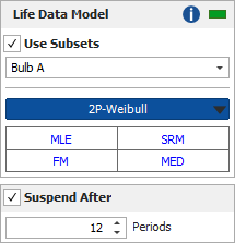
This setting tells the software to look at the information in the subset ID column and separately analyze the data based on their subset IDs. In addition, it allows you to use the drop-down list to switch between subset IDs and alter the analysis settings for each one, if appropriate. As a general rule, however, the recommendation is to use the same analysis settings for all subsets. You select the following analysis settings for each subset ID:
- 2P-Weibull
- Maximum Likelihood Estimation (MLE)
- Standard Ranking Method (SRM)
- Median Ranks (MED)
- Fisher Matrix Confidence Bounds (FM)
Next, you select the Suspend After check box and enter 12 periods.
Note: Most product warranties are of a certain duration, and in many cases data after the warranty period are incomplete or unreliable. The Suspend After check box allows you to specify a period beyond which the data are considered incomplete. For example, consider a shipment that has been in the field for 14 months. If the warranty period is 12 months, then the failures entered in the data sheet for months 13 and 14 are taken into account, but all remaining units in that shipment period are suspended at 12 months.
Once the settings are finalized, you analyze the data sheet by clicking the Calculate icon on the control panel.
![]()
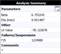
The Analysis Summary area of the control panel will display two sets of parameters (because the data sheet contains two subsets IDs). You view the parameters of each set by choosing the subset ID from the drop-down list, as shown next. The following picture shows the 2P-Weibull parameters of bulb B.

The following picture shows the 2P-Weibull parameters of bulb A.
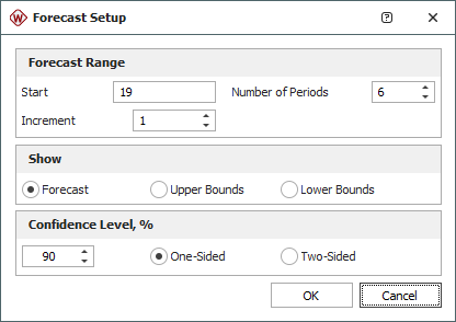
With the analysis completed, the next step is to generate the forecast. You do so by clicking the Forecast icon on the control panel.
![]()
In the setup window, you set the forecast to start on the 19th month and show 6 periods.
The forecast is then generated within the folio and displayed in the data sheet called "Forecast."
On the control panel of the Forecast sheet, you select the Show Subset ID check box in order to identify which type of bulb the expected failure will be. You also select the Use Warranty Length check box, enter 12 periods and click Update.
Note: By default, the software assumes an infinite warranty period. The Use Warranty Length check box allows you to limit the length of the warranty period. In this example, the warranty length is 12, which means that any units that fail after 12 months of operation are not counted in the returns as they are assumed to be out of warranty.
The following Forecast sheet shows the results of your analysis, with the Show Subset ID and Use Warranty Length options selected.

The columns represent the warranty returns periods and the rows represent the sales periods. The results indicate, for example, that you would expect to see a total of 616 bulb failures in the 19th month (column 19), and that 32 of those failures will be from bulb A (as shown in rows 13 to 15), while the remaining failures will be from bulb B. The rest of the forecast can be read in a similar manner.
For our optional analysis task, we want to check whether the assumption of a usage rate of 50 hours/month is valid. The data from the in-house test of bulb B are in terms of hours, so you first convert the data for bulb B according to the hour-to-month ratio (by dividing the failure and suspension times by 50).
You create a new Weibull++ life data folio and manually enter the converted data (here, "Bulb B - In-House Data - Months"). You analyze the data sheet using the same analysis settings that were used on the in-house test data (i.e., 2P-Weibull and RRX). The following picture shows the result of the analysis (for reference, the Subset ID column shows the failure times in terms of hours).

| State F or S |
Time to F or S (mon) |
Subset ID 1 |
| F | 6 | 300 |
| F | 8.8 | 440 |
| F | 9.9 | 495 |
| S | 10 | 500 |
| S | 10 | 500 |
You can now compare the results from the warranty analysis to the results from the in-house test and verify the assumption of the usage rate. One way to do this is to display the contour plot of both data sets and analyses on the same plot.
You create an overlay plot by choosing Home > Insert > Overlay Plot.
![]()
When prompted to select which data sets to plot, you select the converted data set from the in-house test and the data set from the warranty analysis of bulb B (here, "Bulb B - In-House Data - Months" and "Warranty - Bulbs").
On the control panel of the plot sheet, you switch the plot type to a Contour Plot. When prompted to specify the contour lines, you select the 2nd Level, 90% and the 5th Level, 75% check boxes.
The following overlay plot shows that all the contours overlap; therefore, the two data sets do not show a statistically significant difference in the life and the 50 hour/month assumption is valid. (This assumes that the only factor is the hour-to-month ratio and that there is no differentiation between the test and use conditions.)
