Life Data Analysis
In life data analysis, the goal is to model and understand the failure rate behavior of a particular item, process or product. The models are built by taking the observed "life" data, which can be obtained either from the field or from in-house testing. Because time is a common measure of product life, the life data points are often called times-to-failure data. There are two general types of times-to-failure data: complete and censored.
In this example, you will work with these types of data and use the Weibull++ life data folio to perform life data analysis.
Complete Data
You receive a request from a team of product engineers who are working on the design of a projector that your company manufactures. You are asked to quantify the life characteristics of the projector bulb in order to understand its reliability. You are given a data set for 10 bulbs that were all tested to failure by the bulb’s supplier. The test included shutdown and cooldown periods that were intended to simulate normal use conditions. The failure times were 513, 649, 740, 814, 880, 944, 1009, 1078, 1161 and 1282 hours. These failure times are called complete data.
Complete Data: The simplest case of life data is a data set where the failure time of each specimen in the sample is known. This type of data set is referred to as complete data, and is obtained by recording the exact times when each unit failed.
Objectives
- Estimate the average life of the bulb (i.e., MTTF or mean life).
- Estimate the B10 life of the bulbs (i.e., the time by which 10% of the bulbs will be failed, or the time by which there is a 10% probability that a bulb will fail).
- Estimate the reliability of the bulbs after 200 hours of operation.
- Assuming 1,000 bulbs will be fielded, estimate how many would fail after 200 hours.
- Estimate the warranty time for the bulb if you do not want failures during the warranty period to exceed 2%.
MTTF and MTBF: The terms MTBF (mean time between failures) and MTTF (mean time to failure) have often been interchangeably used to describe the average time to failure. The truth is, these two metrics are not the same and should not be used interchangeably.
When dealing with non-repairable components (as in the case of life data analysis) the metric sought is the mean time to failure or MTTF. It is only when dealing with repairable components (where the component may fail and be repaired multiple times during its operational life) that you calculate the mean time between failures or MTBF. The only time that the MTTF and MTBF are the same is when the failure rate is constant (i.e., when the underlying model is an exponential distribution).
Solution
To answer the questions of interest to the design team, you will perform life data analysis on the complete data set provided by the supplier.
First, you create a new Weibull++ life data folio by choosing Home > Insert > Life Data.
![]()
When prompted to specify the data type, you select Times-to-failure data and clear all the other options. You also use the Units drop-down list to indicate that the time values in the data sheet will be entered in hours.
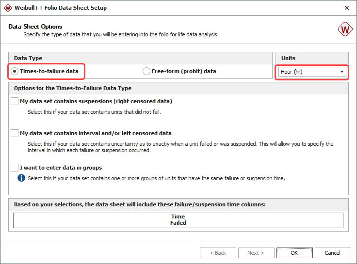
Note: By clearing all the other options, you limit the number of columns that require data entry. In this example, there is no need to select any of the other options because your data set contains only complete data.
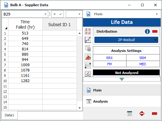
When the data folio has been created, you enter the data given by the bulb supplier.
(You’ll notice that in the screenshots here, we’ve called this folio "Bulb A – Supplier Data." If you want to rename your new folio, right-click the name in the current project explorer and choose Rename.)
|
Time Failed (hr) |
|
513 |
|
649 |
|
740 |
|
814 |
|
880 |
|
944 |
|
1009 |
|
1078 |
|
1161 |
|
1282 |
Note: The new folio starts with a single data sheet by default. You can add multiple data sheets to the folio as needed. Think of the data folio as an Excel® workbook that can contain multiple worksheets.
Once the data set is entered, the next step is to set up the analysis. The analysis options are available in the Analysis Settings area of the control panel. This area provides a quick summary of the settings that will be used to fit a distribution to the data set. The current settings on the Main page of the control panel are as follows:
- Rank Regression on X (RRX)
- Standard Ranking Method (SRM)
- Median Ranks (MED)
- Fisher Matrix Confidence Bounds (FM)
These settings are also available on the Analysis page of the control panel, which can be accessed by clicking the Analysis button, as shown next.
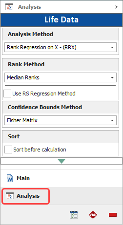
Tip: Instead of switching between control panel pages, you can click the blue text in the Analysis Settings area on the Main page as a quick method for switching between available analysis options.
The next step is to set the distribution that you want to fit to the data. In order to determine which distribution will work best with your data, you click the Distribution Wizard icon on the Main page of the control panel.
![]()
You select to consider all the distributions and then click Analyze to see which of the selected distributions best fits the data set, based on the selected analysis method (in this case, it is for the RRX analysis method).
Note: The Distribution Wizard serves only as a guide. You should compare its results with your own engineering knowledge about the product being modeled before making the final decision on which distribution to use for your data set.
The G-Gamma distribution receives the highest ranking, but you do not recognize this distribution, and based on the analysis details the 2P-Weibull distribution performed nearly as well, and its parameters are more interpretable and explainable. You decide to use the 2P-Weibull distribution, which received the second highest ranking. You close the Wizard and then select 2P-Weibull from the distribution drop-down list on the control panel.
To analyze the data (i.e., fit the selected distribution based on the selected analysis settings), you click the Calculate icon on the control panel.
![]()
Once the distribution is fitted, the Analysis Summary area of the control panel displays the parameters of the distribution and other relevant information. In this case, based on the 2P-Weibull distribution setting, the results are as shown next.

This result includes the Rho, which is the correlation coefficient, and the LK Value, which is the value of the log-likelihood function based on the current parameter solution.
You can now access additional information, obtain metrics and/or view plots. To create a probability plot, you click the Plot icon on the control panel.
![]()
Probability Plots: The Weibull probability plot is drawn on a "Weibull probability plotting paper" that displays time on the x-axis using a logarithmic scale and the probability of failure on the y-axis using a double log reciprocal scale. From the plot, you can obtain the probability of failure at a given time or vice versa.
To obtain the results from the plot, you click the plot line. This displays crosshairs that show the current location on the line. You can move the mouse pointer to track the coordinates from any position on the line. You click the plot again to return to normal mode.
The following example shows the Weibull probability plot with the approximate B10 life of the bulbs (where the x-axis value corresponds to y=10%).
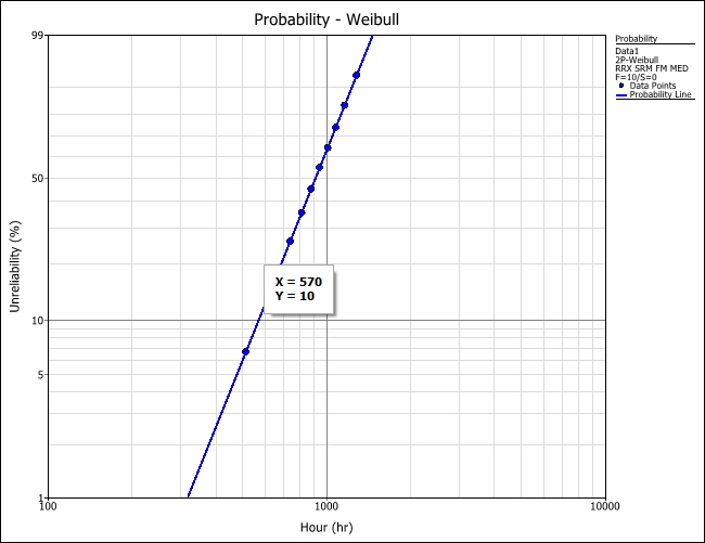
To add a label that displays the coordinates on the plot, you simultaneously press CTRL and ALT, then click a point on the plot.

You find that one of the disadvantages of reading results off the plot is that it may be difficult to position the pointer at exact values. To get more precise results, you open the Quick Calculation Pad (QCP) by clicking the icon on the control panel.
![]()
The QCP provides quick access to a set of commonly needed results. To estimate the MTTF, you select to calculate the Mean Life and use the Units drop-down list to make sure that the results will be returned in hours. You click Calculate. The average time to failure for the bulbs is about 906 hours.
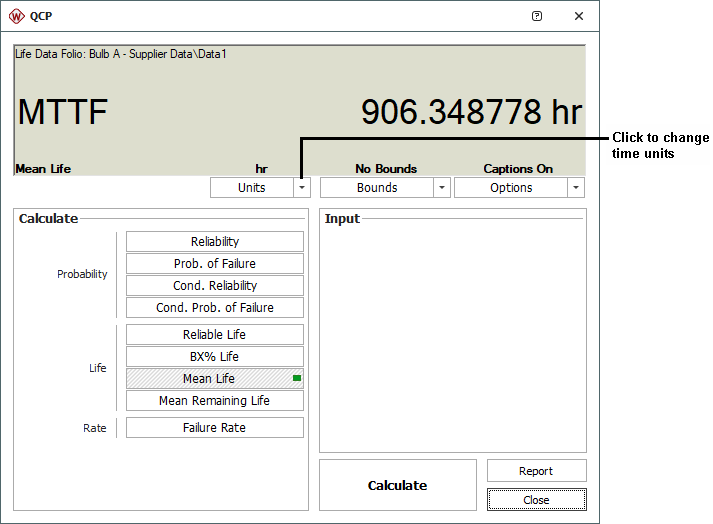
Note: The picture shows the QCP without the optional "Calculation Log" on the right side of the window. To hide or display this log on your computer, click the Options button and then toggle the Show Calculation Log option.
Similarly, you use the QCP to answer the remaining questions:
- To estimate the B10 life, you select to calculate the BX% Life and enter 10 for the BX% Life At input. The result is about 570 hours. A B10 of approximately 570 hours means that 10% of the population will be failed by 570 hours of operation.
- You select Reliability to calculate the reliability at 200 hours. The result is 0.998406 or 99.84%.
- To determine the number of bulbs out of 1,000 that would fail after 200 hours of operation, you first find the probability of failure at 200 hours by selecting Prob. of Failure and entering 200 for the time. The probability of failure is 0.001594 or 0.16%. You multiply this by the total number of bulbs (1,000). The number of bulbs that would fail is 1.6 or approximately 2.
- To estimate the warranty time during which no more than 2% of the bulbs will fail, you select to calculate the Reliable Life and enter 0.98 for the Required Reliability input. The result is about 377 hours. (Alternatively, the same result could have been obtained by calculating the B2 life.)
Censored Data
After analyzing the supplier’s data, you decide that you would feel a lot more comfortable if you could validate the results yourself by performing an in-house test.
After putting in the appropriate requests, you are allocated 15 bulbs for testing purposes and have approval to use the lab facilities for a maximum of 40 days. Unfortunately, only five pieces of equipment that are capable of detecting bulb failures are available for you to use. Given this constraint, you decide to test 5 bulbs using the available automated equipment and test the remaining 10 bulbs via manual inspection. You stop by the lab on your way to your office every morning at 8:00 am (except on weekends and holidays) to check the status of the 10 bulbs. When you find that one of the bulbs has failed, the only information you have is that it failed sometime after you last checked on the bulbs (the last inspection) and before now (the current inspection). This information is called interval censored data.
Censored Data: Censored data means data with missing information. When a unit has failed between observations and the exact time to failure is unknown, the time intervals in which the failures occurred are referred to as interval censored data. On the other hand, for non-failed units that continue to operate after the observation period has ended, the observed operating times of the units are referred to as right censored data or suspensions.
Once the test is completed (after 40 days or 960 hours), you have the following data:
- For the automated equipment, bulbs 1, 2 and 3 failed at 425, 730 and 870 hours respectively, while bulbs 4 and 5 continued to operate after 960 hours.
- For the manual inspections, you have the log shown next, where * indicates a working bulb and X indicates a failed bulb.
| Day | Hrs | Bulb 6 | Bulb 7 | Bulb 8 | Bulb 9 | Bulb 10 | Bulb 11 | Bulb 12 | Bulb 13 | Bulb 14 | Bulb 15 |
| 1 | 24 | * | * | * | * | * | * | * | * | * | * |
| 2 | 48 | * | * | * | * | * | * | * | * | * | * |
| 3 | 72 | * | * | * | * | * | * | * | * | * | * |
| 4 | 96 | * | * | * | * | * | * | * | * | * | * |
| 5 | 120 | * | * | * | * | * | * | * | * | * | * |
| 6 | 144 | Weekend | |||||||||
| 7 | 168 | ||||||||||
| 8 | 192 | * | * | * | * | * | * | * | * | * | * |
| 9 | 216 | * | * | * | * | * | * | * | * | * | * |
| 10 | 240 | * | * | * | * | * | * | * | * | * | * |
| 11 | 264 | * | * | * | * | * | * | * | * | * | * |
| 12 | 288 | * | * | * | * | * | * | * | * | * | * |
| 13 | 312 | Weekend | |||||||||
| 14 | 336 | ||||||||||
| 15 | 360 | * | * | * | * | * | * | * | * | * | * |
| 16 | 384 | * | * | * | * | * | * | * | * | * | * |
| 17 | 408 | * | * | * | * | * | * | * | * | * | * |
| 18 | 432 | * | * | * | * | * | * | * | * | * | * |
| 19 | 456 | * | * | * | * | * | * | * | * | * | * |
| 20 | 480 | Weekend | |||||||||
| 21 | 504 | ||||||||||
| 22 | 528 | * | * | * | * | * | * | * | * | * | * |
| 23 | 552 | * | * | * | * | * | * | * | * | * | * |
| 24 | 576 | * | * | * | * | * | * | * | * | * | * |
| 25 | 600 | * | * | * | * | * | * | * | * | * | * |
| 26 | 624 | * | * | * | * | * | * | * | X | * | * |
| 27 | 648 | Weekend | |||||||||
| 28 | 672 | ||||||||||
| 29 | 696 | * | * | X | * | * | * | * | * | * | |
| 30 | 720 | * | * | * | * | * | * | * | * | ||
| 31 | 744 | * | * | * | * | * | * | * | * | ||
| 32 | 768 | * | * | * | * | * | * | X | * | ||
| 33 | 792 | * | * | * | * | * | * | * | |||
| 34 | 816 | Weekend | |||||||||
| 35 | 840 | ||||||||||
| 36 | 864 | * | * | * | * | * | X | * | |||
| 37 | 888 | * | * | * | * | * | * | ||||
| 38 | 912 | * | * | * | * | * | X | ||||
| 39 | 936 | * | * | * | * | * | |||||
| 40 | 960 | * | X | * | * | * | |||||
Objectives
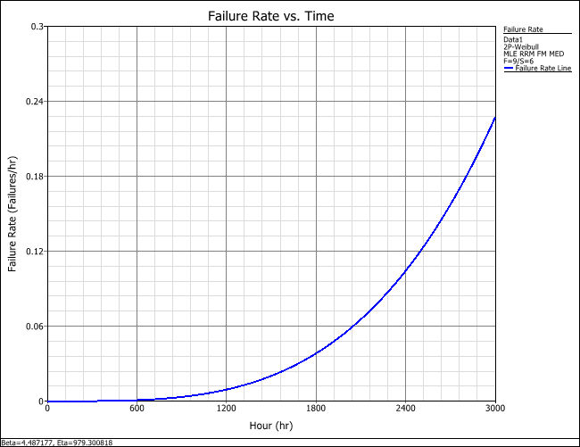
- Use a Failure Rate vs. Time plot to ascertain the failure rate behavior of the bulbs. Your expectation is that the bulbs should have an increasing failure rate. Basically, an increasing failure rate implies an underlying degradation mechanism with time, or in other words, the older the bulb the more likely it is to fail.
- Estimate the average bulb life.
- Estimate the B10 life of the bulbs.
- Estimate the reliability of the bulbs for 200 hours of operation.
- Assuming 1,000 bulbs will be fielded, estimate how many would fail after 200 hours.
- Estimate the warranty time for the bulb if you do not want failures during the warranty period to exceed 2%.
Solution
To answer the questions of interest, you will perform life data analysis on the censored data set that you obtained from both parts of the in-house test (automated equipment and manual inspection).
First, you create a new Weibull++ life data folio (here, we have called it "Bulb A - In-House Data"). When prompted to specify the data type, you select Times-to-failure data and the following check boxes:
- My data set contains suspensions (right-censored data)
- My data set contains interval and/or left censored data
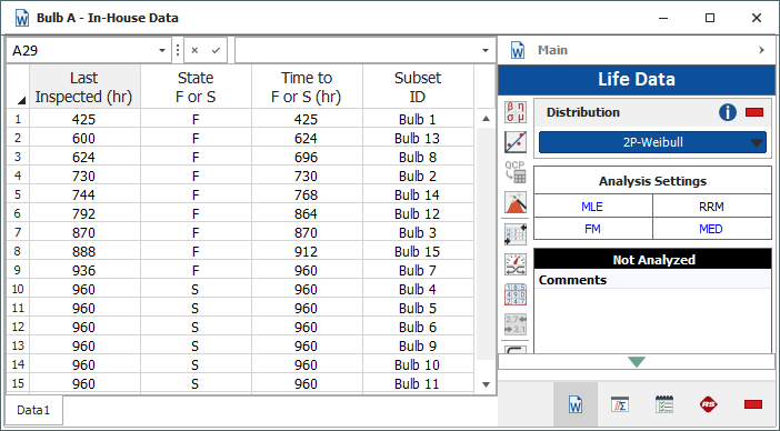
Once the folio is created, you enter the data obtained from both parts of the test in the data sheet. On the control panel, you choose the 2P-Weibull distribution and the MLE parameter estimation method. The resulting data sheet is shown next.
| Last Inspected (hr) | State F or S |
Time to F or S (hr) |
Subset ID |
| 425 | F | 425 | Bulb 1 |
| 600 | F | 624 | Bulb 13 |
| 624 | F | 696 | Bulb 8 |
| 730 | F | 730 | Bulb 2 |
| 744 | F | 768 | Bulb 14 |
| 792 | F | 864 | Bulb 12 |
| 870 | F | 870 | Bulb 3 |
| 888 | F | 912 | Bulb 15 |
| 936 | F | 960 | Bulb 7 |
| 960 | S | 960 | Bulb 4 |
| 960 | S | 960 | Bulb 5 |
| 960 | S | 960 | Bulb 6 |
| 960 | S | 960 | Bulb 9 |
| 960 | S | 960 | Bulb 10 |
| 960 | S | 960 | Bulb 11 |
Maximum Likelihood Estimation (MLE): As a rule of thumb, analysts often use the MLE analysis method when dealing with heavily censored data, as in this example. This is because the MLE method is based on the likelihood function, which considers the time-to-suspension data points in the estimate of the parameters, whereas in rank regression (RRX and RRY) the solution is based on the plotting positions of the times-to-failure data.
Next, you click Calculate to analyze the data set, and then click Plot to create a probability plot.
On the control panel of the plot sheet, you use the Plot Type drop-down list to choose the Failure Rate vs. Time plot. This displays the failure rate behavior of the bulbs over time. The plot shows an increasing failure rate.
Using the QCP as before, you again answer the rest of the questions:
- Mean Life = 893 hours.
- B10 Life = 593 hours.
- Reliability at 200 hours = 0.999194 or 99.92%.
- Probability of failure at 200 hours = 0.000806 or 0.08%. Therefore, when multiplied by 1,000 bulbs, the number of bulbs that would fail is 0.8 or about 1 bulb.
- Warranty time = 410 hours.
Confidence Intervals
Before you submit the results of the in-house test for the projector bulbs, you want to quantify the error that may be associated with your predictions. After all, the results were based on a sample of only 15 bulbs. If you were to repeat the same experiment with another set of 15 bulbs, you would, in all likelihood, obtain different results. To quantify the error due to sampling, you will use confidence intervals (or confidence bounds), which may be viewed as the range of probable values that you are likely to obtain if you were to keep repeating the same experiment with different samples of 15 bulbs, all belonging to the same homogeneous population.
One-Sided or Two-Sided Confidence Bounds: Confidence bounds may be one-sided or two-sided. They are usually around a computed metric, such as the reliability at a given time. Two-sided bounds are used to indicate that the metric of interest is contained within these bounds with a probability equal to the chosen confidence value. For example, 90% two-sided confidence bounds indicate that the metric of interest will be between the bounds 90% of the time, and that 5% of the time it may be above the upper bound and 5% of the time it may be below the lower bound. Another way to express this is to say that the metric of interest will lie between the bounds with a 90% probability.
One-sided bounds, on the other hand, are used to indicate that the metric of interest is above the lower bound with a probability equal to the chosen confidence value. For example, a 90% lower one-sided confidence bound indicates that the metric of interest will be higher than the lower bound with a 90% probability.
An estimated metric that is obtained without the use of confidence bounds is said to be at the 50% confidence level, meaning that error on either side of the estimate is equally probable.
You use the QCP to calculate the MTTF of the bulb. To obtain the desired confidence bounds, you choose Two-Sided from the Bounds drop-down list and enter 0.90 for the Confidence Level input. The calculated results are shown next.

Therefore, with a 90% probability, the true value of the MTTF is estimated to be between 790 and 1,010 hours. While unlikely, there is still a 5% probability that the MTTF is less than 790 hours and a 5% probability that it is greater than 1,010 hours.
To visualize the confidence bounds, you create a Weibull probability plot. To show the bounds, you right-click the plot sheet and choose Confidence Bounds. You then select to display the Two-sided bounds. The following plot shows the 90% two-sided confidence bounds on the Weibull probability plot. Here, the scaling has been adjusted to Y = 0.1 to 99 and X = 100 to 10,000. To do this on your plot, in the Scaling area of the control panel, clear the check boxes for the x- and y-axes to turn off automatic scaling and enter your desired minimum and maximum values for each axis. The new scaling will be shown when you redraw the plot.

Comparing Data Sets
After analyzing the data from the bulb supplier and the in-house test, it would be reasonable to wonder how they compare. Specifically, you want to understand how the data and analysis from the in-house test compare to the data and analysis provided by the bulb supplier. One way to do this is to use an overlay plot that displays both data sets and analyses on the same plot.
You create the overlay plot by choosing Home > Insert > Overlay Plot.
![]()
When prompted to select which data sets to plot, you select the folio containing the data set from the supplier and the folio containing the data set from the in-house test. (here, "Bulb A - Supplier Data" and "Bulb A - In-House Data".)
The following overlay plot shows the two data sets plotted on the same Weibull probability plot (and both with 90% two-sided confidence bounds):
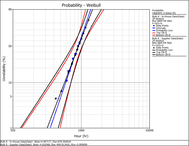
The overlay plot shows that the probability lines of the two data sets have similar slopes. Furthermore, there is a significant overlap in the confidence bounds of both sets, which suggests that both data sets exhibit the same reliability characteristics.
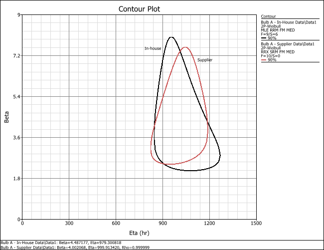
Another way to determine whether there is a statistically significant difference between the two data sets at a given confidence level (say 90% confidence level for this example), is to switch the plot type to a Contour Plot. When prompted to specify the contour lines, you select the 2nd Level, 90% check box.
Tip: To add contour lines (confidence levels) to the plot or change the confidence level associated with a contour line, click the Contours Setup link on the control panel of the plot sheet.
You add labels to the plot by holding down the CTRL key and then clicking in the plot. You then edit the text by double-clicking the labels. To position the text on the plot, you click the label and then drag it by its handle (i.e., the small box on the upper left corner of the label).

The annotated plot is displayed next (with the scaling adjusted to Y = 0 to 9 and X = 0 to 1,500). The contour plot shows that the two data sets overlap at the 90% confidence level; therefore, they do not show a statistically significant difference at that confidence level.
Reports
For presentation to the rest of the team, you will prepare a report that summarizes the results of your analyses. Weibull++’s built-in reporting tool, the ReliaSoft Workbook, combines two reporting modules: spreadsheet and word processing.
Objectives
- Use the spreadsheet module to calculate all of the results that you obtained individually from the QCP.
- Use the word processing module to create a document that presents the key results, along with a plot of the failure rate vs. time.
Spreadsheet Module
You create a ReliaSoft Workbook by choosing Home > Insert > ReliaSoft Workbook.
![]()
When prompted to specify a default data source, you choose the folio containing the bulb supplier’s data (here, "Bulb A - Supplier Data") and click OK to create a blank workbook.
In the workbook, you click the Spreadsheet button in the Modules panel and build a worksheet like the one shown next. You use the Function Wizard to build functions that automatically insert calculated results based on the specified data source.
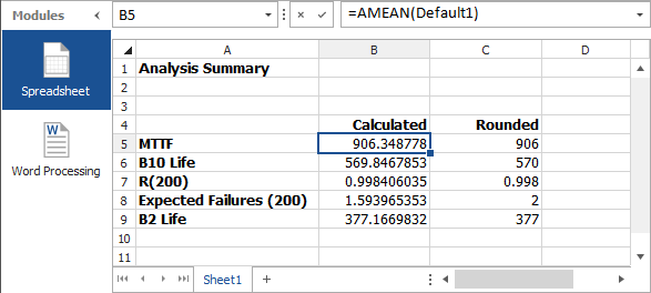
For example, to build the function that is highlighted in the picture, you open the Function Wizard by choosing Home > Report > Function Wizard.
![]()
You select the AMEAN function from the list.
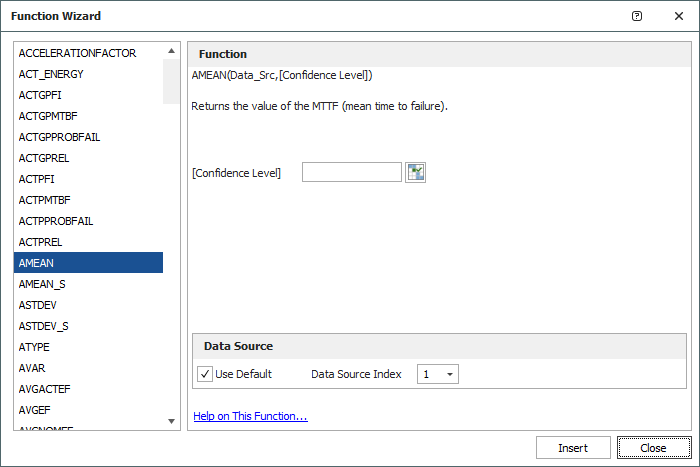
The confidence level input is optional (as indicated by the brackets that enclose the label) and not applicable in this example. So you simply specify the data source by selecting the Use Default check box. From the Data Source Index drop-down list, you select the number 1 (i.e., the first default data source, which you selected when you created the workbook), then you click Insert.
The MTTF for the specified data set will be automatically computed and displayed in the workbook. You continue to use the Function Wizard to build the rest of the report:
- To calculate the B10 life, you select the TIMEATPF function and enter 0.1 for the Unreliability input.
- To calculate the reliability at 200 hours, you select the RELIABILITY function and enter 200 for the Age input.
- To calculate the expected number of failures after 200 hours of operation, you first calculate the probability of failure and then multiply that number by the total number of bulbs (1,000 bulbs in this example). To do this, you enter the following formula directly into the appropriate cell: =(1 - B7)* 1000, where B7 is the cell reference of the reliability at 200 hours, as shown in the picture earlier.
- To calculate the B2 life (which is equivalent to the warranty time during which no more than 2% of the bulbs will fail), you select the TIMEATPF function and enter 0.02 for the Unreliability input.
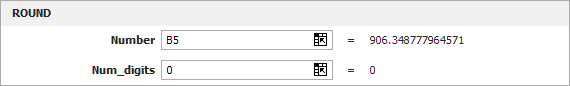
To round the numbers to the nearest integer, you use a math function. You choose Formulas > Function Library > Insert Function.
![]()
You select ROUND from the list and click OK. When prompted to define the function arguments, you enter B5, which is the cell reference to the first calculated result; and 0 (zero), which indicates that you will be rounding the number to the nearest integer.
In the worksheet, you copy this formula by clicking inside cell C5 and then dragging the fill handle (small black square on the lower right of the cell) down the column of cells.
You review the resulting worksheet and notice that the value in cell C7 appears to be equal to 1. To change its rounding precision, you double-click the cell and edit its function to use three decimal places: = ROUND(B7,3). You press ENTER to save the changes.
Word Processing Module
Next, you click the Word Processing button in the Modules panel and build a report template like the one shown next. You use the Function Wizard and Plot Wizard to insert functions into the desired locations.
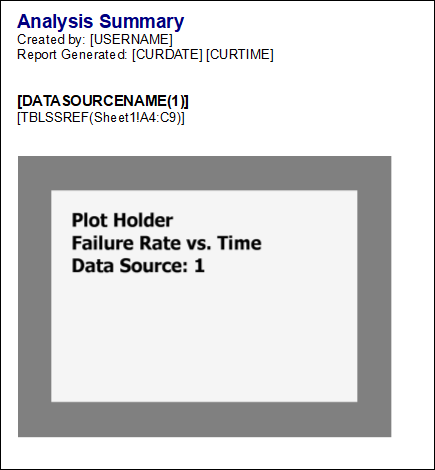
For example, to insert the display name of the person who generates the report, you open the Function Wizard and select the User Name function from the list. You continue to use the Function Wizard to build the rest of the report:
- To insert the date and time that the report is generated, you select the Current Date and Current Time functions.
- To insert the name of the life data folio and data sheet that the results will be pulled from, you select the Data Source Name function. You also select the number 1 for the data source index.
- To insert the results that you created in the spreadsheet module, you select the Spreadsheet Reference function. You then click the Select button next to the Cell Reference field and, when prompted to select cells, you highlight the table that contains the calculated results (cells A4 to C9) and click OK.

Tip: You can also access the Spreadsheet Reference function from the ribbon while in the word processing module by choosing Home > Report > Spreadsheet Reference.
To insert the Failure Rate vs. Time plot, you open the Plot Wizard by choosing Home > Report > Plot Wizard.
![]()
You select the Failure Rate vs. Time plot from the list. You also select the number 1 for the data source index. You then click Insert to add a placeholder for the plot.
To resize the plot, you select its placeholder, and then click and drag the resize handles (i.e., the small circles that appear within the corners of the selected placeholder).
When you have finished building the report template, you click the Review tab at the bottom of the window. This generates a preview of the report, with all the data and plots inserted.
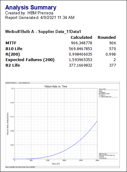
You generate the final report in Microsoft Word by returning to the design view and choosing Home > Report > Send to Word.
![]()
Tip: If you want to create the same reports for the bulb’s in-house data set, you could simply change the first default data source assigned to the workbook (Home > Report > Associate Data Sources). Alternatively, if you want to compare both data sets in the same report, you can add a second default date source and then duplicate/modify the functions. For example, use =RELIABILITY(Default1, 200) to return the reliability from the supplier data set and create a new function =RELIABILITY(Default2, 200) to return the reliability from the in-house data set.