Design of Reliability Tests

Weibull++ includes several test design tools that provide ways to design reliability tests and evaluate/compare proposed test designs. In this example, you will work with two tools available in the Test Design folio.

You'll start by using the Reliability Demonstration Test tool to design a zero-failure test intended to demonstrate a specified reliability for a projector bulb titled "Bulb A." Afterwards, you’ll use the Expected Failure Times Plot to compare the failure times that are expected from a design with a specified reliability to the actual failure times that are observed during a test.

Combining the Test Data for Bulb A

In order to design a reliability demonstration test, we generally need an estimate of the failure rate behavior. This can come from field data for similar components, a test conducted on a prototype or even an educated guess. If there is limited or no information available, we can try several such guesses and choose the most conservative resultant test plan.

In this scenario, we have already analyzed some test data from bulb A, and the analysis shows that the failure behavior of bulb A follows a 2-parameter Weibull distribution with beta = 4.22.

Reliability Demonstration Test Design

Based on your past experience with bulb A, which we plan to use in an upcoming projector model, you are asked to design a demonstration/validation test to show that the bulb has the required B10 life of 500 hours. This is equivalent to 90% reliability at 500 hours.

More specifically, your objective is to demonstrate that bulb A has a B10 life of at least 500 hours with 80% confidence. You are allocated 10 bulbs for the test and decide on a zero-failure reliability demonstration test. In other words, you decide to design a test that uses the available sample size of 10 and will demonstrate the target metric if no failures occur before a certain time (i.e., you design a test where the number of "allowable" failures is zero).

Zero-Failure Tests: A zero-failure test is appropriate in this case because you only want to know, with a given confidence level, whether the life metric is greater than the specified requirement. This sort of test provides a quick and efficient way of accomplishing this. Note, however, that zero-failure tests generally cannot be used to determine the actual value of a product’s life metric. (In some special cases, the 1-parameter Weibull or 1-parameter exponential distribution can be suitable for analyzing a data set containing few or no failures.) Further, if our estimate of the failure rate behavior is not accurate, we will have no way of knowing based on the results of a 0 failure test.

Objectives

Determine the test time for a zero-failure test that would demonstrate the target metric with a sample size of 10.
Compare the test times that would be required given different sample sizes and different numbers of "allowable" failures.

Solution

To create a new test design folio, you choose Home > Insert > Test Design.

In the Test Design Assistant window, you select Reliability Demonstration Test Design. Since you are able to make reasonable assumptions about the life distribution that describes bulb A’s failure rate behavior, you select the Parametric Binomial test design method on the control panel of the folio. To specify the metric that you wish to demonstrate, you choose Reliability value at a specific time from the Metric drop-down list on the RDT sheet. Then you enter 90 for the reliability and 80 for the confidence level. (The B10 life is equivalent to the time at which reliability reaches 90%.)

In the At this time field you enter 500, which is the time at which you want to demonstrate this metric. Based on your previous experience, you choose a Distribution of 2P-Weibull and enter 4.22 for the With this Beta value.

In the Solve for this value area, you select to solve for the Required test time for a test with a sample size of 10. To specify that this will be a zero-failure test, you enter 0 for the maximum number of failures. Finally, you click the Calculate icon.

(You’ll notice that in the screenshots here, we’ve called this folio "Zero-Failure Test - Bulb A." If you want to rename your new folio, right-click the name in the current project explorer and choose Rename.)

The inputs and results appear as shown next.

Based on this calculated result, you need to test the 10 bulbs for at least 553 hours each. If no failures occur during that time, you will have demonstrated that the bulb has a B10 life of at least 500 hours with 80% confidence (i.e., if no failures occur before about 553 hours, then there is an 80% probability that the B10 life is greater than 500 hours).

You would also like to explore the possibility of using a different sample size and examining the sample size’s effect on test time. This may allow you to find a better combination of sample size and test time. So you click the Show RDT Table icon on the control panel.

A sheet called "Table of RDT 1" is added to the folio. You select to solve for the Test time for given sample size and specify that you want to see the required test times for sample sizes that range from 5 to 20, using an increment of 1. Then, because you want to view test times for zero-failure and 1-failure tests, you specify that you want to consider numbers of failures that range from 0 to 1. Finally, you click Generate Table and see the results shown next.

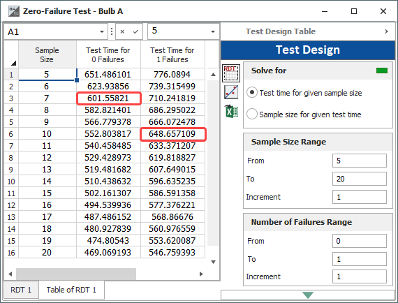
This table uses the target metric and life distribution information you provided earlier to calculate the test times needed under many different scenarios. For example, the first highlighted cell shows that you could reduce the sample size to 7 and test to 602 hours instead of 553 (with zero failures). The second highlighted cell shows that if you were to stay with your current sample size of 10, you could demonstrate the target metric even if 1 failure occurred. However, the required test time in that case would increase to 649 hours.

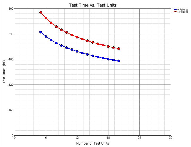
To more easily see how sample size, test time and number of failures are related, you generate a plot of this information by clicking the Plot icon.

Expected Failure Times Plot

Before performing a reliability life test, you can use the Expected Failure Times Plot to provide an overall expected timeline and sequence of events for the test based on an expected life distribution. This in turn can be used during the actual test to monitor its progress for any early warnings that indicate a deviation from the original assumptions or expectations.

After a discussion with management, you are asked to go ahead and run a life test on five bulbs of a different model titled bulb B.

Objectives

Use the Expected Failure Times Plot to determine what range of failure times you can expect to observe on each unit of bulb B during this test, assuming that it follows the same life distribution as bulb A, that is 2P-Weibull with beta = 4.22, eta =991 hrs.
As the units of bulb B begin to fail during the test, compare the failure times to the expected times. If the bulbs appear to differ in life distribution, determine which has a greater B10 life.

Solution

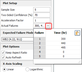
To create the plot, you choose Home > Insert > Test Design and select Expected Failure Times Plot in the Test Design Assistant. In the Plot Setup area on the control panel, you enter 5 for the sample size and 70 to specify that you wish to see 70% two-sided confidence bounds for each expected failure time. You enter 1 for the acceleration factor because the units will be tested under normal stress conditions.

You need to specify a reliability model for the expected life distribution. To do this, expand the Expected Failure Model drop-down and specify Beta to be 4.22, Eta to be 991 and the units to be Hours, then click OK.

The information in the Expected Failure Model area of the control panel is now updated with the distribution and parameters that we just entered. Alternatively, you could select from published reliability models. Click the Redraw Plot icon to display the ranges of expected failure times. Here, the scaling has been adjusted to X = 0 to 1,300. To do this on your plot, in the Scaling area of the control panel, clear the check box for the x-axis to turn off automatic scaling and enter your desired minimum and maximum values for the x-axis. The new scaling will be shown when you redraw the plot.

This plot uses the failure number on the y-axis (1 = the first failure, and so on) and time on the x-axis. Based on the plot, you expect the first failure to occur sometime between 440 and 787 hours of testing, the second between 635 and 928 hours, and so forth. You view the actual time bounds by pointing to the first or last tick mark on a line, as shown next for the first failure.

The Expected Failure Times Plot: In general, this plot tells you that, based on the assumed distribution, you can expect the observed failure times to be within the ranges shown. If any sequential observed time is outside this range, then the distribution (and thus the reliability) of the observed units should no longer be assumed. (The plots results are only valid, however, for the confidence level chosen.) Moreover, if any of the observed failure times is earlier than its predicted interval, then you can infer that the reliability will be less than what was assumed. Similarly, if any of the actual failure times is greater than its predicted interval, then you can infer that the reliability is greater than what was assumed (at the specified confidence level).

As the test progresses, you observe the first failure at 300 hours, which is earlier than the associated starting interval. You conclude that, at the specified confidence level, bulb B’s reliability is less than what was assumed. In order to estimate the bulb’s B10 life, you continue the test to collect more data. The next 2 failures are observed at 440 and 495 hours. As these failures occur, you display them on the plot by clicking inside the Actual Failures field on the control panel and entering them into the table that appears. After recording these 3 failures, the table appears as shown next.

The plot appears as shown next.

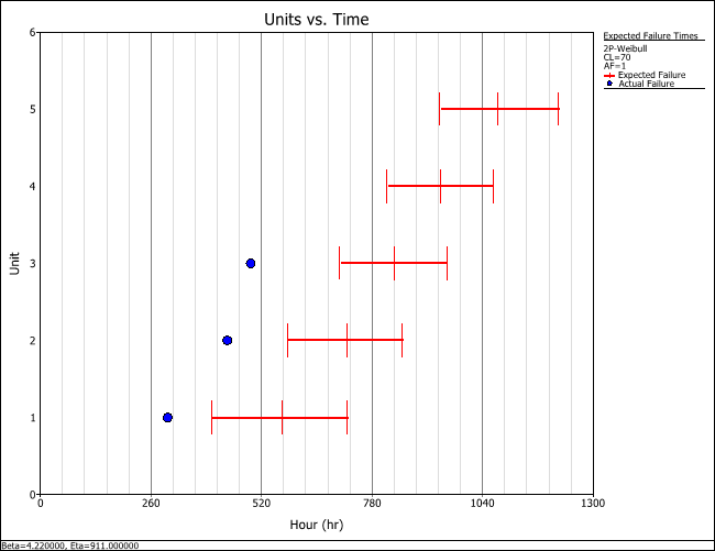
With three failure times observed, it is clear that the reliability of bulb B is lower than that of bulb A, so we end the test at 500 hours instead of expending additional resources. We may wish to calculate the parameters of bulb B’s life distribution based on these failure times and compare them to any data from bulb A.