Difference Detection Matrix
The Difference Detection Matrix calculates how much test time is required before it is possible to detect a statistically significant difference in the mean life or BX% life (e.g., B10 life) of two product designs by analyzing the data from a reliability life test. You can use this tool to evaluate different test plans in order to choose the one that will be most efficient to compare the reliability of the two designs. To use the matrix, you must provide various inputs—including the sample sizes that will be used to test each design and the life distributions that describe each design’s life behavior.
The ReliaWiki resource portal has more information on the Difference Detection Matrix at: http://www.reliawiki.com/index.php/Reliability Test Design.
Reading the Detection Matrix
In this section, we will look at an example detection matrix and discuss how to read it. The next section explains how to set up the matrix. We will assume that a sample size of 10 will be used to test both product designs.
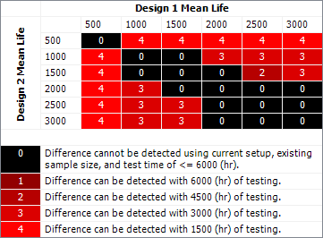
Because the column title in the above matrix is "Design 1 Mean Life," we know that the metric being compared is mean life (rather than BX% life). The column headings represent possible mean life values for Design 1, and the row headings represent possible mean life values for Design 2. We’ll begin by examining the cell in the second column and the first row of the matrix, which corresponds to a Design 1 mean life of 1,000 hours and a Design 2 mean life of 500 hours.
The number inside this cell is 4 and the legend below the matrix tells us that a 4 means a difference between the two designs can be detected, but only after at least 1,500 hours of testing. In other words, one thing the matrix tells us is that if Design 1 has a mean life of 1,000 hours and Design 2 has a mean life of 500 hours, then the tests we use to compare these designs will need a duration of at least 1,500 hours in order for the analysis of collected data to show that there is, at the specified confidence level, a statistically significant difference in mean life between the two designs.
Tip: You can click a cell in the matrix to see the difference in the compared metric that was calculated for both designs based on the associated test time. For example, if a cell in the matrix shows that a difference in mean life can be detected with 2,000 hours of testing, clicking the cell will show the mean life calculations (including two-sided confidence intervals) that would be obtained for each design if you analyzed the test data after 2,000 hours of testing. (If only one of the designs would produce enough failures to fit to a distribution during the given test time, no intervals will be shown.)
Setting Up the Detection Matrix
Follow the steps outlined below to set up the detection matrix. All the settings are located on the control panel.
- In the Metric to Compare
area, select whether you want to compare Mean
Life or BX% Life.
If you select to compare the BX% life, you must enter a value
in the associated input field (e.g., a BX% life of 10 indicates
that the software will compare the time when 10% of units
will have failed). Also, specify the confidence level that
will define when a difference between the specified designs
is statistically significant. Then specify the time units
(e.g., hours) that will be used for the inputs and results.
The software calculates two-sided confidence intervals (at the level you specified in the Confidence (%) field) on the specified life metric for both designs, when possible. A difference is considered detected at a given test time when the two calculated confidence intervals do not overlap, or when only one of the designs produces enough failures to fit to a distribution. - In the Design 1 and Design 2 areas, enter the sample sizes of the tests that will be used to compare the designs and define the distributions for each design’s failure behavior.
- In the Reliability
Metric Setup area, configure the rows and columns in
the table by first entering the Max
Metric Time value, which is the highest metric value
(mean life or BX% life, depending on your selected metric)
that the software will consider in the comparison. Then enter
a Metric Increment
to specify the difference between the displayed metric values
in each column and each row. This value is also used as the
minimum metric value that will be considered in the comparison.
For example, if you entered 1000 in the Max Metric Value field and 200 in the Metric Increment field, then your matrix would have five columns and five rows, each starting with a value of 200 and moving up in increments of 200 until reaching the maximum value of 1000.

- The matrix indicates whether a difference in the selected
reliability metric will be detected after various test times.
These are the test times shown in the legend under the matrix.
In the Test Times Matrix
Setup area, specify the test times that will be evaluated.
- To specify how many test times to evaluate, enter a value in the Number of Test Times field. For example, if you enter 4 in this field, then the software will evaluate will evaluate 4 different test times. The software cannot evaluate more than 10 test times.
- If the Calculate Test Times check box is cleared, you will be able to click the arrow inside the Test Time field to open a table where you can enter the specific times. For example, if you enter 500 as one of the test times, then the matrix will determine whether 500 hours (assuming your selected time unit is hours) is sufficient to detect a difference in the selected life characteristic. The number of rows available in this table is determined by what you entered in the Number of Test Times field. Note that upon exiting the table, the times in the table will be sorted in descending order.
- If the Calculate Test Times check box is selected, the software will automatically enter test times from 1,500 to 6,000 in the Test Time field.
- Click the Calculate
icon to validate your settings and generate the matrix. See
Reading
the Detection Matrix for information on how to read the
results.
- If you wish to export the matrix as a Microsoft Excel file, click the Send to Excel icon.
![]()
- You can also change the color used in the matrix by clicking the Set Matrix Color icon.
![]()
Your selected color will be used to indicate when the shortest test time provided in the Test Time Matrix Setup area is sufficient to detect a difference in the specified life characteristic. Darker versions of that color will be used to indicate when longer test times are required.