Repairable Systems SimuMatic Folio
For reliability growth data analysis only.
The Repairable Systems SimuMatic folio gives you access to the generated data sets and to the results of analyses performed automatically for those data sets.
Simulation Sheet
The Simulation sheet shows the parameters calculated for each data set. It also contains a separate column for each of the calculations that you specified on the Analysis and Results tabs of the setup window. The following columns may be included in the Simulation sheet, depending on the metrics you chose to calculate in the Repairable Systems SimuMatic Setup window.
- Beta and Lambda of the Crow-AMSAA model are the calculated parameters for each data set.
- The following values are calculated according to the
inputs you provided on the Analysis tab of the setup window.
- Target DMTBF is the time required to demonstrate the specified MTBF.
- DMTBF is the demonstrated MTBF at the end of the test.
- DFI is the demonstrated failure intensity at the end of the test.
- Growth Rate is equal to 1 - beta. A larger growth rate means faster MTBF growth.
- The following values are calculated according to the
inputs you provided on the Results tab of the setup window.
- IMTBF(t) and CMTBF(t) are the instantaneous/cumulative MTBF at a specified time, t.
- T_IMTBF(m) and T_CMTBF(m) are the time given a specified instantaneous/cumulative MTBF, m.
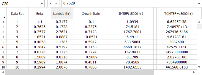
As an example, the following picture shows the results from the first ten data sets for a particular simulation. In this case, the analysts chose to display only the Crow-AMSAA model parameters (Beta and Lambda), the growth rate, the instantaneous MTBF at 15,000 hours (IMTBF(15000) and the lower confidence bound on the time at which the demonstrated MTBF reached a specified target value (Target DMTBF).
Sorted Sheet
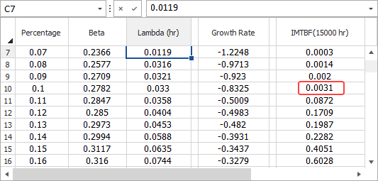
In the Sorted sheet, the calculated values from the Simulation sheet are sorted from least to greatest in order to show the confidence bounds. The Percentage column displays the percentage of data sets that are equal to or less than a given data set. So, for example, if you wished to obtain the 90% lower one-sided confidence bound on the instantaneous MTBF at 15,000 hours, you would look up the value of IMTBF(15000) (hr) that corresponds to 10% (i.e., 100% - 90%), as shown next.
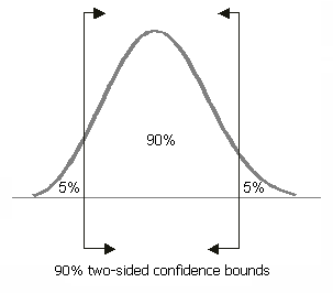
Alternatively, if you wished to obtain the 90% two-sided confidence bounds of IMTBF(15,000), you would look up the values that correspond to 5% (for the lower bound) and 95% (for the upper bound), as illustrated in the next figure.
Control Panel
The SimuMatic control panel and its components are described next,
- The Model area always displays "Crow-AMSAA (NHPP)" because this is the only model Reliability Growth SimuMatic uses to generate simulated data.
- The Analysis Settings table shows what settings were used in the analysis of each data set. These settings will vary depending on the data type selected.
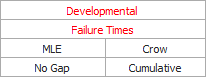
As an example, the following picture shows the settings that are used for the Failure Times data type. The settings show the type of data (Developmental – Failure Times), parameter estimation method (MLE), confidence bounds method (Crow), whether a gap interval has been defined in the analysis (No Gap) and whether the failure times are entered as cumulative or non-cumulative (Cumulative).
- The Parameters area displays the Crow-AMSAA model parameters that were used to generate the data.
- In the Additional Results
area:
- The T(i) (...) button opens a report that displays each data set in its own column. (Note that this report will contain multiple sheets when there are too many data points to fit onto one sheet.)
- The Summary (...) button opens a report that displays the settings used to generate the data. It also displays the average and median parameter values of the data sets.
The following tools are available on the SimuMatic control panel:
![]() SimuMatic Setup
allows you to change your simulation settings and replace your
current simulated data sets with new ones.
SimuMatic Setup
allows you to change your simulation settings and replace your
current simulated data sets with new ones.
![]() Plot generates
the Plot sheet, which allows you to view the five different plots
based on the simulated data.
Plot generates
the Plot sheet, which allows you to view the five different plots
based on the simulated data.
Plot Sheet
In the plot sheet, five different kinds of plots are available in the Plot Type drop-down list on the control panel.
- Cumulative Number of Failures gives an indication of how the number of failures is increasing over time. It plots the times on the x-axis and the cumulative number of failures on the y-axis. The points represent the actual failure times in the data set, and the solution line represents the expected cumulative number of failures based on the calculated model parameters. The vertical line represents the test termination time.
- The Cumulative
MTBF vs. Time and Instantaneous
MTBF vs. Time plots show how the time between consecutive
failures increases, decreases or remains constant over time.
- The cumulative MTBF is the MTBF from time = 0 up to a given end time. For example, a cumulative MTBF of 5 hours from 0 to 100 hours means that, on average, the time between failures was 5 hours over the 100-hour period.
- The instantaneous MTBF is the MTBF over a small interval dt that begins at a given time. For example, an instantaneous MTBF of 5 hours at 100 hours duration means that, over the next small interval dt that begins at 100 hours, the average MTBF will be 5 hours.
- The Cumulative Failure
Intensity and Instantaneous
Failure Intensity plots show how the failure intensity
changes over time.
- The cumulative failure intensity is the average failure intensity from the beginning of the test (i.e., t=0) up to a given time.
- The instantaneous failure intensity is the failure intensity over a small interval dt that begins at a given time.
The following options on the plot sheet are unique to SimuMatic plots. They allow you to control which elements will be displayed on the plot. See Plot Utilities for more general information on plot sheets.
- Simulation Lines plots the line (e.g., cumulative MTBF vs. time) for every simulated data set.
- True Parameter Line plots the line defined by the parameters of the Crow-AMSAA model. (These parameters are visible on the control panel of the Simulation sheet.)
- Median Line and Average Line plots the lines defined by the median and average parameters of all generated data sets.
- CB on Function and CB on Time plot two-sided confidence bounds on the plot. The "Function" is determined by the current plot type (e.g., cumulative MTBF is the function for the cumulative MTBF vs. time plot). The percentile of the confidence bounds is determined by what you entered for Confidence Bounds on Plot on the Analysis tab of the setup window.
- Target is available when you have selected the Calculate Target Time option on the Analysis tab of the setup window. This option marks the target time on the instantaneous MTBF/FI vs. time plots.