Parametric RDA Folio Control Panel Settings
The parametric RDA folio control panel allows you to configure the analysis settings for the data sheet and view/access the results. This topic focuses on the Main page and Analysis page of the parametric RDA folio control panel, which contain most of the tools you will need to perform the analysis. For more information about the control panel in general, see Control Panels.
Control Panel Main Page
The GRP model uses the concept of virtual age to mathematically capture the effect of the repairs on the subsequent rate of occurrence of failure (i.e., failure intensity). The rate of occurrence of failure over time is modeled by the power law function. This means that the GRP analysis method has three parameters, two of which are used to describe the power law function and a third for estimating the virtual age of a system.
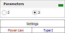
- The Parameters area allows you to select how you want to calculate the parameters of the GRP model. If you select 2 parameters, you will be prompted to specify a value for the virtual age parameter based on your own knowledge about the effectiveness of the repairs (this may be the q or RF parameter, depending on your default setting). If you select3parameters, the software will calculate the virtual age parameter based on the data, giving you an indication of the effectiveness of the repairs as reflected by the data set.
- The Settings area displays "Power Law" to indicate that the power law function will be used in the analysis. This setting cannot be changed; however, you have the option to select which virtual age model will be used in the analysis. Click the option displayed in blue text on the control panel to toggle between the available virtual age models.
- The Analysis Summary
area displays the calculated results. The following example
shows the calculated values of the parameters and the likelihood
(LK) value of the GRP model for a particular data set. You
can click the Detailed Summary
icon
 to open the
Results window, which shows the results in a worksheet that
you can copy or print.
to open the
Results window, which shows the results in a worksheet that
you can copy or print.

Folio Tools
The folio tools are arranged on the left side of the Main page of the control panel:
![]() Calculate
estimates the parameters of the GRP model, based on the current
data set. This tool is also available by choosing Recurrent
Event Data > Analysis > Calculate.
Calculate
estimates the parameters of the GRP model, based on the current
data set. This tool is also available by choosing Recurrent
Event Data > Analysis > Calculate.
![]() Plot creates
a new sheet in the folio that provides a choice of applicable
plot types. In parametric RDA folios, this includes cumulative
failures vs. time, failure intensity vs. time, etc. This tool
is also available by choosing Recurrent
Event Data > Analysis > Plot.
Plot creates
a new sheet in the folio that provides a choice of applicable
plot types. In parametric RDA folios, this includes cumulative
failures vs. time, failure intensity vs. time, etc. This tool
is also available by choosing Recurrent
Event Data > Analysis > Plot.
![]() QCP opens
the Quick Calculation
Pad, which allows you to calculate results based on the analyzed
data sheet, such as the number of failures and mean time between
failures (MTBF). This tool is also available by choosing Recurrent Event Data > Analysis
> Quick Calculation Pad.
QCP opens
the Quick Calculation
Pad, which allows you to calculate results based on the analyzed
data sheet, such as the number of failures and mean time between
failures (MTBF). This tool is also available by choosing Recurrent Event Data > Analysis
> Quick Calculation Pad.
![]() Change Units
opens the Change Units window,
which allows you to change the units for the values in the current
data sheet. This tool
is also available by choosing Recurrent
Event Data > Format and View> Change Units
Change Units
opens the Change Units window,
which allows you to change the units for the values in the current
data sheet. This tool
is also available by choosing Recurrent
Event Data > Format and View> Change Units
Control Panel Analysis Page
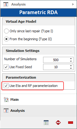
The following settings are available on the Analysis page of the parametric RDA control panel:
- The Virtual Age Model
area allows you to select one of two ways that the GRP model
can calculate the virtual age after each repair:
- Only since last repair (Type I) assumes that the repairs will remove some portion of the damage that has accumulated since the last repair.
- From the beginning (Type II) assumes that the repairs will remove a portion of all the damage that has accumulated since the system was new.
- The Simulation Settings
are for the Monte Carlo simulation. In general, the application
uses the failure times supplied by the data set in order to
calculate virtual age. However, when extrapolating for results
that are outside of the range of observations, the failure
times are unknown. Therefore, unless the virtual age parameter
q = 1, there are
no analytical solutions available for metrics such as total
failure number and failure intensity. In this case, the solution
can be obtained only through Monte Carlo simulation.
- The Number of Simulations specifies the number of data points to generate in the simulation.
- The Use a Fixed Seed checkbox is an optional setting that allows you to specify a starting point from which random numbers are generated in the simulation. The same random numbers and, therefore, the same simulation results will be generated when the same seed value and number of data points are used.
- The Parameterization option allows you to select how you want the parameters to be calculated. By default, the software calculates for the beta, lambda and q parameters. However, if you want to publish the model and use it in BlockSim, then you need to express the power law parameter (lambda) in terms of the Weibull parameter (eta) and express the virtual age parameter (q) in terms of the RF parameter (which users of BlockSim will recognize as the restoration factor of a maintenance action). To do this, select the check box in the Parameterization area, as shown next.
The ReliaWiki resource portal explains the mathematical concept behind these two models at: http://www.reliawiki.org/index.php/Imperfect Repairs. (Note that the article is written for ReliaSoft's BlockSim software, but the theory remains the same.)
Since it may not be feasible to classify real-world repair situations into one of these two abstract categories, the virtual age type is usually selected based on what provides a better statistical fit for the data. The model fit can be assessed by using the likelihood (LK) value that is displayed in the Analysis Summary area on the control panel, where the higher value indicates the better fit.
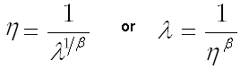
The relationship between the power law parameter, lambda (λ), and the Weibull parameter, eta (η), is described as:
The relationship between the q and RF parameters is described as:
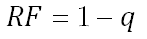
The RF parameter indicates the degree to which the condition of a system will be restored after each repair. Parameter q indicates the opposite. A value between 0 and 1 indicates the extent of the repair, where:
- An RF = 1 indicates that the system will be "as good as new" after the repair. This is also called perfect repair.
- An RF value between 0 and 1 indicates that the system will be "better than old but worse than new" after the repair. This is also called imperfect repair.
- An RF = 0 indicates that the system will be "as bad as old" (i.e., no improvement) after the repair. This is also called minimal repair.