Example: Multi-Phase Test Planning and Management

For reliability growth data analysis only.

The data set used in this example is available in the example database installed with the software (called "Weibull22_ReliabilityGrowth_Examples.rsgz22"). To access this database file, choose File > Help, click Open Examples Folder, then browse for the file in the Weibull sub-folder.

The name of the project is "Multi-Phase Test Planning and Management."

A manufacturer is developing a small electric vehicle for indoor use, such as airports. The goal MTBF for the vehicle is 300 operating hours. 20 developmental prototypes are going to be tested for 3,000 hours each, for a total of 60,000 hours. The first phase of testing is planned to end at 5,000 hours of cumulative test time; the second phase will end at 15,000 hours; the third phase will end at 25,000 hours; the fourth will end at 35,000 hours; the fifth will end at 45,000 hours and the sixth will end at 60,000 hours.

The analysts wish to:

• Create a test plan that will achieve the desired MTBF goal.
• Use the Crow Extended - Continuous Evaluation model to analyze the data at the end of each phase of testing.
• Use the multi-phase plot to track the actual progress against the original test plan.

Continuous Growth Planning Folio

The first step of creating an overall reliability growth program plan is to set an idealized growth curve and planned MTBF goal at each stage of the program. This will help determine the management strategy that may be needed to achieve the final MTBF goal. (The reliability growth program plan for this example is located in the growth planning folio called "Test Plan.") The inputs on the data sheet are shown next.

 

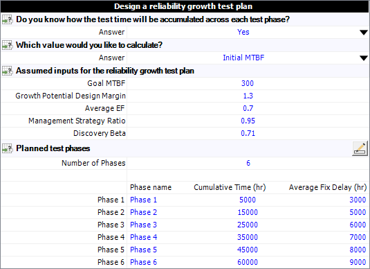
You can see that the cumulative test time at the end of each test phase has been defined under the Planned test phases heading, along with the average fix delay for failure modes that are discovered in each phase. In this case, the team expects that it will be easier to implement fixes earlier in the process; therefore, the estimated fix delay increases in each phase. For example, the fix for a failure mode discovered during Phase 1 is expected to be implemented approximately 3,000 test hours later; whereas a failure mode discovered during Phase 5 might not be able to be fixed until approximately 8,000 test hours later because the design is more mature at that point.

The growth planning folio also shows the inputs for the Crow Extended growth planning model. In this case, the analysts have selected to calculate for the Initial MTBF that the product must have before reliability growth testing begins in order to achieve the Goal MTBF of 300 hours by the end of the test program, given the following growth management strategy:

• A GP Design Margin of 1.3, which indicates that the growth potential MTBF (i.e., the maximum achievable MTBF if you continue until all modes are observed and corrected according to the current maintenance strategy) must equal 130% of the goal MTBF. This value provides a "safety factor" to ensure that the reliability requirement is met.
• An Average EF of 0.7, which indicates that the team expects that the fixes applied to failure modes discovered during testing will remove about 70% of the failure intensity due to those modes.
• A Management Strategy of 0.95, which indicates that the team plans to fix about 95% of the failure modes that are discovered during testing (while about 5% may be classified as A modes, which are not fixed due to technical, financial or other reasons).
• A Discovery Beta of 0.71, which indicates that the inter-arrival times between unique failure modes discovered during testing will become larger as the test progresses.

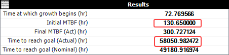
As shown next, the results indicate that the initial MTBF must be about 131 hours when the first test phase begins. Furthermore, the plan estimates that the MTBF goal will be achieved after about 58,000 hours of test time.

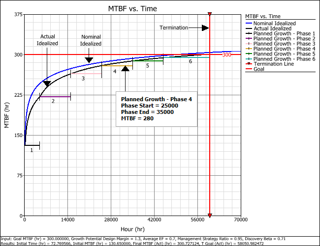
Click the Plot icon to see a visual representation of the results that are expected in each phase of testing. The following picture contains annotations to help you identify the following:

• The Actual Idealized and Nominal Idealized lines show the overall characteristic pattern for the reliability growth across all phases of testing.
  • The actual MTBF takes into account the average fix delay. If fixes are not incorporated instantaneously, the actual line will show slower growth compared to the nominal line.
  • The nominal MTBF is the best case scenario, which assumes that the average fix delay is zero.
• The horizontal Planned Growth lines mark the duration of each test phase, as well as the MTBF that is expected to be achieved by the beginning of the phase. For example, the planned growth line for Phase 4 begins at 25,000 hours, ends at 35,000 hours and shows that the MTBF is planned to be about 280 hours by the beginning of that phase.
• The Goal line marks the MTBF the analysts plan to achieve.
• The Termination line marks the end of the last test phase at 60,000 hours of cumulative test time.

Analyze the Test Data with the Continuous Evaluation Model

When the testing began, the team used the Multi-Phase Failure Times data type in Weibull++ to record the data. For demonstration purposes, the sample project contains separate folios with the data up to the end of each individual test phase. As an example, you can open the "Test Data - Through Phase 2" folio, which contains all of the data through the end of the second phase. The last twenty data points from this folio are shown next.

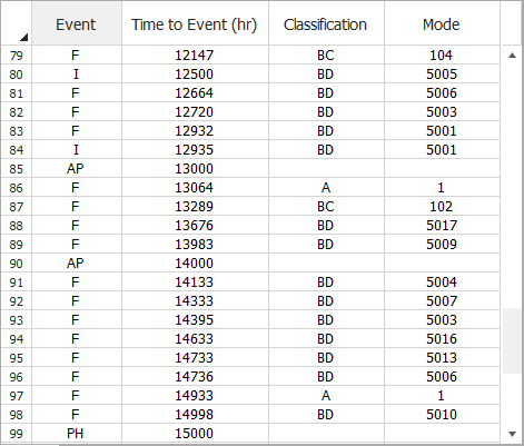
As you can see, in addition to recording the time and mode classification for each failure event (F)—where A = no fix, BC = immediate fix before testing resumes and BD = delayed fix—this data type also allows the team to identify:

• PH: The end time of each phase, which allows for the data from multiple test phases to be entered and analyzed together in the same data sheet.
• I: The specific time when delayed fixes are implemented during testing. For example, on row 84 in this picture, you can see that a fix was applied at 12,935 hours for mode 5001.
• AP: Specific analysis points at which the team wants to calculate results in order to track the progress of the test plan.

(Although they are not shown in this picture, this data type also allows you to mark events as performance (P) or quality (Q) issues that can be excluded from the analysis if desired, You can also mark any event with an X to exclude it from the analysis.)

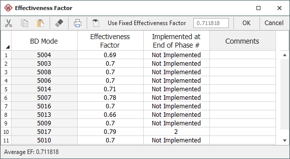
For the BD (delayed fix) failure modes that do not have a specific fix time (I event) recorded in the data set, the Effectiveness Factors window allows the team to specify when the fix was (or will be) implemented. To open the window, choose Growth Data > Crow Extended > Effectiveness Factors.

As you can see, the fix for mode 5017 was implemented at the end of the second phase, and it's expected to have an effectiveness factor of 0.79 (i.e., only 79% of the mode's failure intensity is expected to be removed because the fix is not perfectly effective). The remaining modes have not yet been fixed before the start of Phase 3; they may be fixed during or between later test phases.

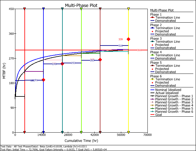
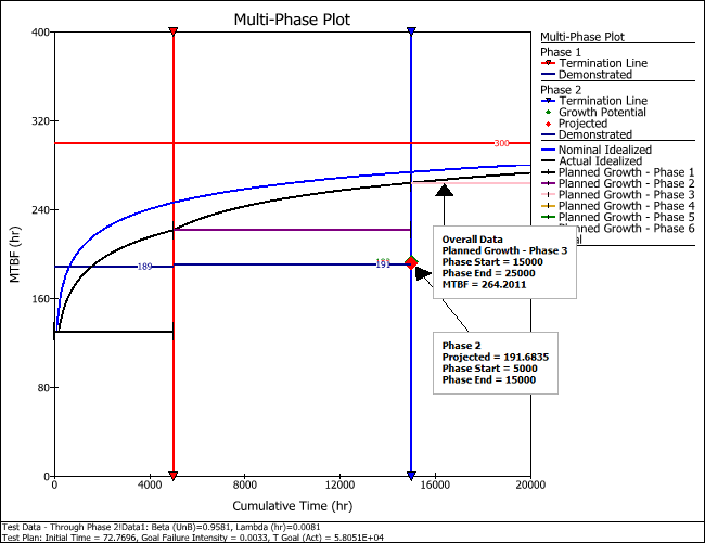
Multi-Phase Plot

As the testing progressed, the team used Weibull++’s multi-phase plot to track the progress against the original test plan. As an example, you can open the "Through Phase 2" multi-phase plot. This plot shows that the MTBF expected after the delayed fixes are implemented after Phase 2 (194.0895 hours) is less than the MTBF planned for the beginning of Phase 3 (264.2011 hours). The team can use this information to determine whether the growth management strategy needs to be adjusted in subsequent phases.

Note: The multi-phase plots in this example are based on analyses that use the maximum likelihood estimation (MLE) method to calculate the parameters, which is known to produce a biased value for beta. In this example, all these plots are based on unbiased estimates of beta. If the folio is not configured to remove this bias, you will be prompted to change the option in the Settings tab of the Item Properties window (Project > Current Item >  Item Properties). To ensure the unbiased beta is always calculated for all new folios, use the RGA Growth Data Folios page of the Application Setup window to select the option.

Finally, if you open the "All Test Phases" multi-phase plot, you can see that the demonstrated MTBF eventually exceeded the goal, indicating a successful reliability growth plan.