Reliability Demonstration Test Design
In a zero-failure reliability demonstration test (RDT), the engineer aims to demonstrate a specified target metric (e.g., reliability at a specific time with a given confidence level) by testing a specified number of units for a predetermined time. If no failures occur, then the target metric is demonstrated. This method has been adapted for scenarios where the target metric can be demonstrated even if some failures occur, as long as a specified number of allowable failures is not exceeded. For example, in a demonstration test where the number of allowable failures is 2, the target metric is demonstrated if no more than 2 failures occur during the test. (If more than the number of allowable failures occurs, then the reliability demonstration test failed and the target metric was not demonstrated. The engineers may choose to continue the test as a reliability life test, recording the exact failure/suspension times and then analyzing the data with standard life data analysis methods. Note that although mathematically it is possible to design a new test with more allowable failures and a longer duration to demonstrate the same target metric, it is unlikely that the metric will be demonstrated by the new test if the original demonstration test failed.)
ReliaSoft's RDT tool can assist the user in designing a demonstration test by solving for various values related to the test, such as sample size, required test time, the demonstrated reliability and the confidence level at which the target reliability will be demonstrated.
Tip: This tool could determine, for example, that if you assume your units follow a Weibull distribution with a shape parameter of 2 and you tested 10 units for 150 hours and none failed during the test, then you would demonstrate a 90% reliability at 100 hours with 90% confidence. It does not, however, calculate the probability that one or more units might actually fail during the test. If you wish to estimate whether a failure is likely to occur, one option is to use the Expected Failure Times Plot to estimate the first failure time based on the assumed distribution and parameters.
Control Panel
- Test Design Method
allows you select a test design option. The method you select
will determine the required inputs on the RDT sheet.
Parametric Binomial determines what test duration or sample size will be required to demonstrate either reliability at a specific time or a specified mean time to failure. To use this option, you must provide an estimate of the underlying life distribution's shape parameter.
Note: You can get the parameters and time units from a calculated data sheet in the current project by clicking the Get Distribution icon
 on the control
panel.
on the control
panel.- If you are demonstrating the reliability at a specified time, enter the time in the At this Time field. If you used the Get Distribution option, this value will initially be set to the time at which a product with the calculated life distribution would have the reliability that you specified.
- If you are demonstrating the mean time to failure, enter the mean time in the Demonstrate this MTTF field. If you used the Get Distribution option, this value will initially be set to the MTTF that a product with the calculated life distribution would have.
- You can also create a table that displays a range of test duration values as a function of sample size and number of allowable failures. The table can also display a range of required sample size values as a function of test time and number of allowable failures. After you create this table, you can also create a plot displaying the same information. This provides a quick way to consider many possible test plan scenarios without having to perform each calculation individually.
- Non-Parametric Binomial solves for the demonstrated reliability, confidence level or sample size that is associated with a specified test design. It does not require a life distribution. The use of this option assumes that the time at which the reliability is demonstrated is equal to the specified test time multiplied by the specified acceleration factor. For example, if the acceleration factor is 1, then the time at which reliability is demonstrated equals the test duration. If the acceleration factor is 2, then the time at which the reliability is demonstrated is double the test duration, and so on.
- Exponential Chi-Squared
determines the total accumulated test time that will be
required to demonstrate a specified metric. The total
accumulated test time is equal to the total amount of
time experienced by all of the units on test. For example,
if the total accumulated time is 100 hours, then you could
test 1 unit for 100 hours, or you could test 2 units for
50 hours each, or you could test 5 units for 1 hour each
and 1 unit for 95 hours.
This option is based on the chi-squared distribution, and it is only for products that have an assumed exponential life distribution (i.e., products with a constant failure rate). - Non-Parametric
Bayesian solves for the demonstrated reliability
or confidence level that can be expected from a specified
test design. It can also solve for the sample size needed
to demonstrate a target reliability at a specified confidence
level. To use this option, you must have some prior information
with which you can estimate the product’s reliability.
In the RDT data sheet, you will need to specify whether the source of prior information is expert opinion (i.e., engineering experience) about the reliability of the entire system or prior testing at the subsystem level:- If you have experience regarding the system as a whole, choose Expert opinion on reliability. Then, enter worst case, expected and best case estimates of the product's reliability.
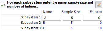
- If you have prior test data for subsystems that compose your system, choose Prior tests at the subsystem level, and then specify the number of subsystems that you will enter data for. You can enter the information for each subsystem in the RDT sheet or click the Edit Bayesian Subsystems icon to open a window you can use to enter the prior test data.
Like the non-parametric binomial option, the use of the non-parametric Bayesian option assumes that the time at which the reliability is demonstrated is equal to the specified test time multiplied by the specified acceleration factor.
The following chart shows the information that each method can provide. The ReliaWiki resource portal has more information on these methods at: http://www.reliawiki.org/index.php/Reliability_Test_Design.
|
|
Metric to demonstrate: |
Can solve for: |
|
Parametric Binomial |
The reliability at a specific time |
The test time for a specified sample
size |
|
Non-Parametric Binomial |
Reliability at test time |
The demonstrated reliability |
|
Exponential Chi-Squared |
The reliability at a specific time |
The total accumulated test time |
|
Non-Parametric Bayesian |
Reliability at test time |
The demonstrated reliability |
- Units in the control panel allows you to define the units of time that will be used in the test.
- Display Options is available when you select to solve for sample size. Select the check box to display the sample sizes as integers.
- Acceleration Factor allows you to enter the acceleration factor associated with the stress level that will be used in the test, if applicable. The acceleration factor is obtained by dividing the product’s life at the use stress level by its life at the accelerated stress level to be used in the test, if applicable. For example, if the product has a life of 100 hours at the use stress level and it is being tested at an accelerated stress level which reduces its life to 50 hours, then the acceleration factor is 2. If you are testing units under normal operating conditions, then the acceleration factor is 1.