To calculate a statistical value, select the appropriate function
option on left side of the Function Option page. Then enter the
required inputs and click Calculate.
The following options are available:
 Median
Ranks
Median
Ranks
The Median Ranks option returns the probability of failure
based on the sample size and order number of the failure.
The probability estimates are at a 50% confidence level.
The median rank is obtained by solving the following
equation for Z:
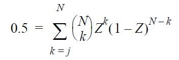
where:
- N is
the sample size.
- j is
the order number.
- Z is
the median rank.
- Other
Ranks
The Other Ranks option returns the probability of failure
based on the sample size and order number of the failure.
The probability estimates are at a confidence level percentage
point that is specified by the user.
The rank is obtained by solving the following equation
for Z:
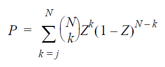
where:
- N is
the sample size.
- j is
the order number.
- P is
the confidence level.
- Z is
the rank.
- Standard
Nominal Values
The Standard Normal Tables option returns the probability
of observing a value less than or equal to x
on the standard normal curve, given a value for x. To find the value
of x given the
probability, use the Inverse Standard Normal Values option.
The probability is obtained by solving the following
equation for Z(x):
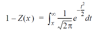
where Z(x) is the probability
of observing a value less than or equal to x.
- Inverse
Standard Normal Values
The Inverse Standard Normal Tables option returns a
value for x on
the standard normal curve, given the probability of observing
a value less than or equal to x.
To find the probability given x,
use the Standard Normal Tables option.
The output is obtained by solving the following equation
for x:
where Z(x) is the probability
of observing a value less than or equal to x.
- Cumulative
Poisson
The Cumulative Poisson option returns the probability
of an event occurring n
times during a specified interval. The required inputs
are n and the
average rate of occurrence for the event, λ,
where λ > 0.
The probability is obtained by solving for P(n, λ)
in the following equation:
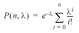
where:
- n is
the maximum number of occurrences (and the upper limit
of the summation).
- λ is
the average rate of occurrence for the event.
- Cumulative
Binomial Probability
The Cumulative Binomial Probability option returns the
probability of an event occurring k
or more times in N
trials. The required inputs are k,
N and the probability
(entered as a decimal number) of the event occurring per
trial.
The probability is obtained by solving for P
in the following equation:
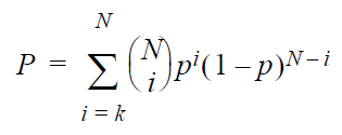
where:
- P is
the probability of the event occurring k
or more times in N
trials.
- p is
the probability of the event occurring per trial.
- N is
the minimum number of trials (and the end of the summation).
- k is
the minimum number of occurrences (and the starting
point of the summation).
- F-Distribution Values
The F-Distribution
option returns Q(F|n1,n2), the significance
level at which we can reject the hypothesis that one sample
has a smaller variance than another. The three inputs
required are the degrees of freedom for both samples and
the ratio of the observed dispersion of the first sample
to that of the second. To find the ratio of the observed
dispersion, use the Inverse F-Distribution Values option.
The output is obtained by solving for Q(F|n1,n2) in the following equation:
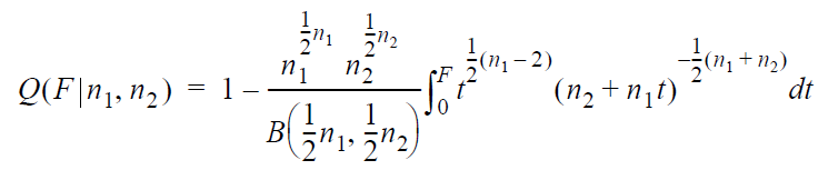
where:
- n1 is the degrees of freedom for the first sample.
- n2 is the degrees of freedom for the second sample.
- F is the ratio of the observed dispersion of the first sample to that of the second.
- B is the beta function.
- Inverse
F-Distribution Values
The Inverse F-Distribution
option returns F,
the ratio of the observed dispersion of one sample to
that of another. The three inputs required are the degrees
of freedom for both samples and the significance level
at which we can reject the hypothesis that the first sample
has a smaller variance than the second. To find the significance
level at which we can reject the hypothesis, use the F-Distribution
Values option.
The output is obtained by solving for F in the following equation:
where:
- n1 is the degrees of freedom for the first sample.
- n2 is the degrees of freedom for the second sample.
- Q(F|n1,n2) is the
significance level at which we can reject the hypothesis
that the first sample has a smaller variance than
the second.
- B is the beta function.
- Chi-Squared
Values
The Chi-Squared Values option returns the chi-squared
value at the (1-d)
percentile. The required inputs are the area to
the right of the critical value and the number of degrees
of freedom.
The output is obtained by solving for  in
the following equation:
in
the following equation:
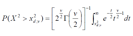
where:
- d is
the area to the right of the critical value.
- v is
the number of degrees of freedom.
- X2
is a chi-squared random variable with v degrees of freedom.
- Incomplete
Beta Function
The Incomplete Beta Function option returns the value
of Ix(a,b).
The required inputs are the values of x,
a and b.
The output is obtained by solving for Ix(a,b)
in the following equation:
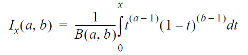
where 0 < x
< 1.
- Gamma
Function
The Gamma Function option returns the value of Γ(n). The only required
input is n.
The output is obtained by solving for Γ(n)
in the following equation:
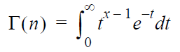
where n >
0.
- Student's
t Values
The Student’s t
Values option returns the t-value
of the Student's t-distribution,
given the probability of observing a value equal or less
than the t-value
and the number of degrees of freedom.
The output is obtains by solving for t
in the following equation:
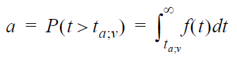
where:
- a is
the probability of observing a value equal to or less
than t.
- v is
the degrees of freedom.