Example of a Nevada Chart Warranty Analysis
The data set used in this example is available in the example database installed with the Weibull++ software (called "Weibull21_Examples.rsgz21"). To access this database file, choose File > Help, click Open Examples Folder, then browse for the file in the Weibull sub-folder.
The name of the project is "Warranty - Nevada Chart Format with Statistical Process Control."
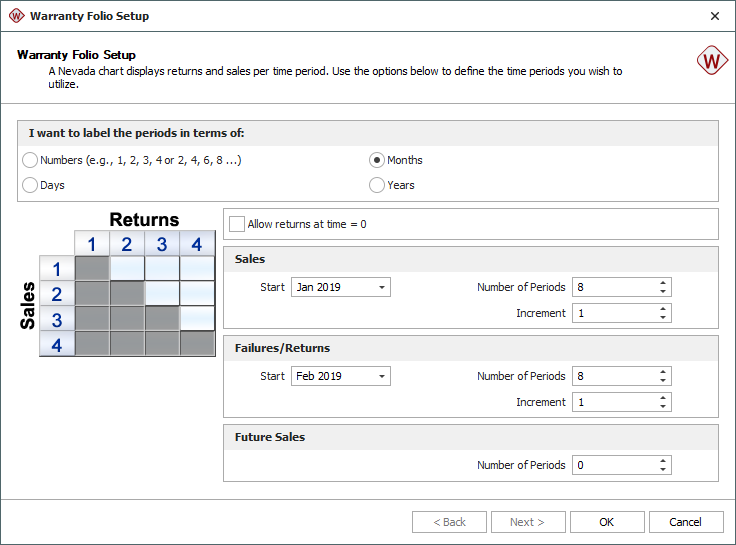
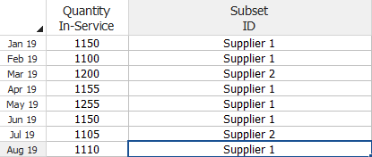
An electronics manufacturer wants to study the expected number of returns for a product they created using materials obtained from two suppliers. The sales and returns data for the product are collected and entered into a Nevada chart warranty analysis folio, as shown next.
Analyze the Data Set Using the Statistical Process Control (SPC) Method
- On the Main page of the control panel, choose the 2P-Weibull distribution and the MLE parameter estimation method.
- On the Statistical Process Control page of the control panel, select the Calculate chi-squared values check box. Make sure that the critical value is 0.01 and that the caution value is 0.1.
- Select the Color-code Returns sheet check box and select the By sales period option.
- Choose Warranty > Analysis > Calculate or click the Calculate icon on the Main page of the control panel.
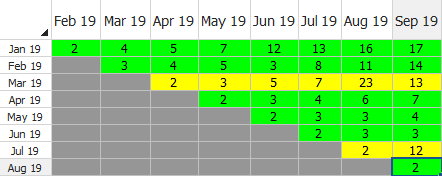
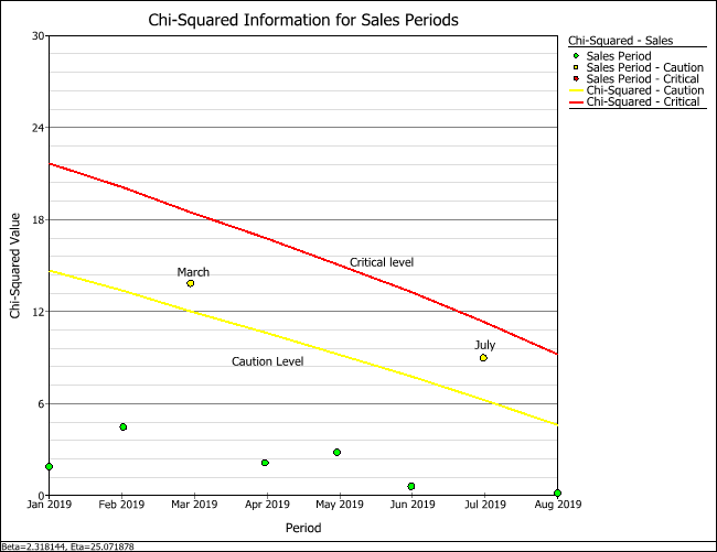
The parameters are estimated to be: beta = 2.3181 and eta = 25.0719. Notice that in the Returns sheet, the March and July sales periods are in yellow. This means that the number of returns for those sales periods is between the caution and critical levels.
- Click the Plot icon. From the Plot Type drop-down list, choose Chi-Squared - Sales. The plot shows that the data points for March and July are between the caution and critical levels. This implies that the population is not homogeneous and that different subpopulations may exist in the data. One suspected reason for the deviation may be the type of material used by the suppliers. The manufacturer concludes that the data set needs to be analyzed based on their material supplier.
Analyze the Data Set Based on Suppliers
- Return to the Sales or Returns data sheet. On the Main page of the control panel, select the Use Subsets check box. Note that selecting this option will make the SPC feature unavailable. For each subset ID, select the2P-Weibulldistribution and theMLEparameter estimation method.
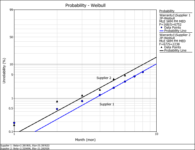
- Click the Calculate icon to recalculate the parameters. The results show that for Supplier 1, the parameters are beta = 2.3819 and eta = 25.3976; for Supplier 2, the parameters are beta = 2.3207 and eta = 21.2829.
- Click the Plot icon. The following plot shows the probability of failure of the two subsets. The plot shows that the material from Supplier 2 tends to have a higher probability of failure compared to the material from Supplier 1.
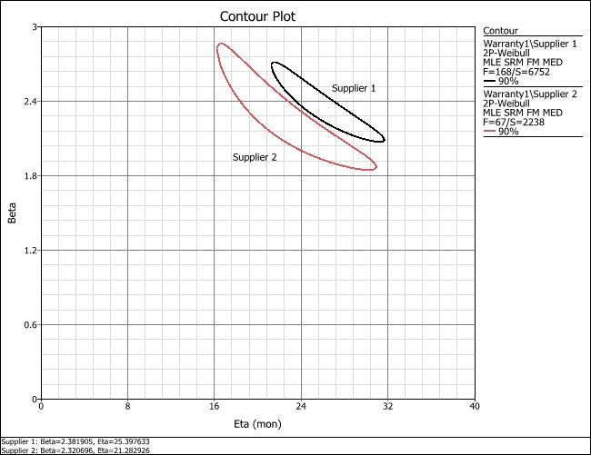
- To determine the statistical difference between the two data sets, create a contour plot. Click the Plot Type drop-down list on the control panel and choose Contour Plot. In the Contour Setup window, select to plot the contours at the 90% confidence level and click OK.
The resulting plot shows that the two subsets do not overlap at the 90% confidence level. This confirms that the two data sets are significantly different at the 90% confidence level.
Generate a Warranty Forecast
The next step is to generate a warranty forecast to obtain the expected number of product returns within a specified warranty period.
- Return to the Sales or Returns data sheet. Choose Warranty > Tools > Forecast or click the icon on the control panel.
![]()
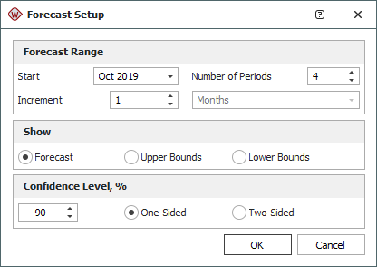
- In the Forecast Setup window, set the forecast range to start in October and end after 4 forecast periods, as shown next. Set the Increment to 1 and click OK.
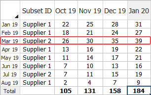
The following figure shows the Forecast sheet with the warranty period starting in October 2019 and ending in January 2020. The results show that the highest number of product returns is expected to come from the batch that was in-service in March.
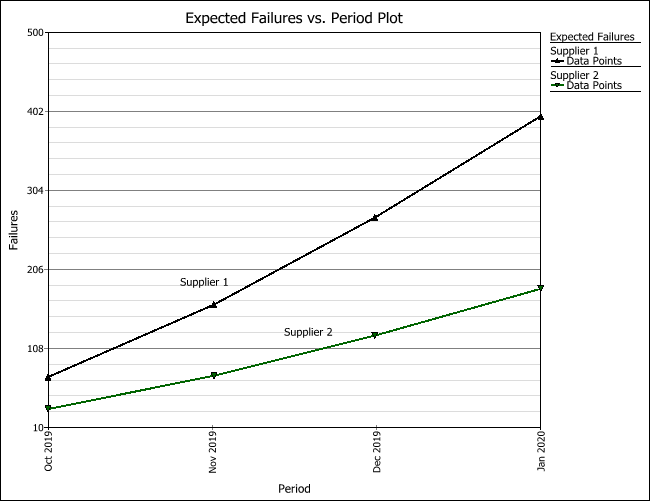
- Click the Plot icon on the control panel of the Forecast sheet. On the Plot Type drop-down list, choose Expected Failures. The following plot shows the expected number of returned units over the warranty period.
Earlier, we found out that the material from Supplier 2 tends to have a higher probability of failure when compared to the material from Supplier 1. However, the current plot shows that Supplier 1 is expected to have a higher number of total returns within the specified warranty period. Looking back at the Sales sheet, we can see that the manufacturer sold three times more units made with materials from Supplier 1 compared to the number of sold units using materials from Supplier 2. Therefore, more units made with the materials from Supplier 1 will be returned each month due to the high sales volume of those units. This forecast analysis can help the manufacturer plan for warranty costs and service, as well as plan for the number of units to produce using materials from each supplier and decide whether it would be worthwhile to have Supplier 2 increase the reliability of its materials.