Estimating Usage

Like any other warranty analysis folio in Weibull++, the usage format must convert the sales/returns data to failures/suspensions that can be analyzed with life data analysis techniques. Since the returns information is entered in terms of accumulated usage (e.g., miles, cycles, etc.) rather than time, the failure "times" will be the usage values recorded when the units were returned. However, an additional step is required to estimate the amount of usage accumulated by the units still operating in the field at the end of the observation period (i.e., the suspensions). Two methods are available for you to provide the information required for these calculations:

• You can define the average amount of usage that any given unit will typically accumulate over a specified period of time (e.g., 500 miles per month, 1,000 cycles per year, etc.).
• You can define a statistical distribution that reflects the variation in usage patterns among different customers. The information for the usage distribution could come from customer surveys, repair records, built-in devices that record usage data, etc.

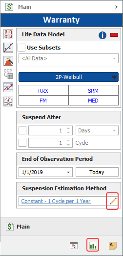
To select a method, click the link in the Suspension Estimation Method area of the Main page or click the Suspensions page icon at the bottom of the control panel, as shown next.

Both methods are described next.

To perform the estimates based on average usage

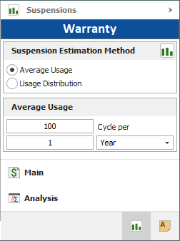
When you choose Average Usage on the Suspensions page of the control panel, you will be required to enter the average amount of usage that any given unit typically accumulates over a specified period of time (in days, months or years). As an alternative, you could have the software calculate the average usage based on the unit conversion factors. For example, the settings shown in the following picture might indicate that the average amount of usage typically accumulated by a washing machine during 1 year of operation is 100 cycles.

When you click the Calculate icon on the Main page of the control panel, Weibull++ will perform the following calculations for each group of units that have the same date in-service:

1. Calculate the number of units from the sales group that were still operating at the end of the observation period:
   
   Number of Units Sold – Number of Units Returned = Number of Suspensions
2. Calculate the amount of time (in days) that those units had been in service by the end of the observation period:
   
   End of Observation Period date – Date In-Service = Days in Service
3. If necessary, convert the average usage to the daily rate for calculation purposes (e.g., if the average usage is 10,000 miles per year, then the daily rate would be approximately 27.3973 miles per day).
4. Estimate the amount of usage the suspension units may have accumulated by the end of the observation period:
   
   Days in Service * Average Usage per Day = Estimated Usage at Time of Suspension

For example, suppose that the Sales sheet records that 50 cars entered service on January 1st while the Returns sheet records the mileage for the 20 units from this sales group that have been returned. If you enter July 1st for the End of Observation Period date and 1000 miles/per year for the Average Usage, the software will calculate the suspensions from the January 1st sales group as follows (where the daily rate has been rounded to 4 decimal places for the sake of simplicity, and therefore the estimated usage will not exactly match the value calculated by the software):

• 50 Units Sold – 20 Units Returned = 30 Suspensions
• July 1 – January 1 = 181 Days in Service
• 181 Days in Service * 2.7397 Miles per Day = 495.8857 Miles approximately

When you click the Show Analysis Summary button on the Main page of the control panel, the life data analysis data set will include one row with 30 suspensions at "End Time" = 495.8857.

To perform the estimates based on a usage distribution

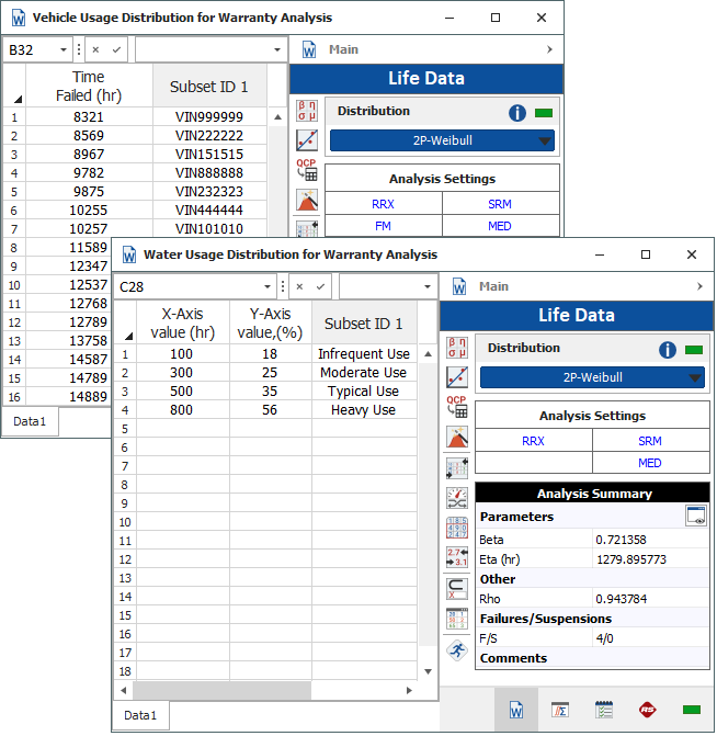
If you have more specific information about variations in usage patterns between different customers, you may prefer to describe the estimated usage in terms of a statistical distribution instead of an average. There are several different ways that you could obtain a usage distribution. For example, if you have information about the amount of usage accumulated by many different users over a specified period of time, you could analyze the data in a Weibull++ life data folio with a time-to-failure data sheet. Alternatively, if you can define typical usage patterns and estimate the percentage of users who are likely to belong to each group (e.g., 18% of customers use 100 cycles or less, 25% of customers use 300 cycles or less, and so on), you could analyze the data in a Weibull++ life data folio with a free-form (probit) data sheet, as shown next.

• When you choose Usage Distribution on the Suspensions page of the control panel, you will be required to define a distribution that reflects the usage amounts that different customers may accumulate during a specified period of time (called the Usage Distribution Period).
  • If you choose Weibull, Normal, Lognormal, Exponential, Generalized Gamma, Gamma, Logistic, Loglogistic or Gumbel from the drop-down list, you can simply enter the appropriate parameter(s) for the selected distribution.
  • If you choose Mixed Weibull, you can use the Subpopulation drop-down list to define parameters and the portion (percentage of the population) represented by each subpopulation.
  • If the estimated values of the distribution parameters are not available, you can use the Quick Parameter Estimator (QPE) to solve for them.
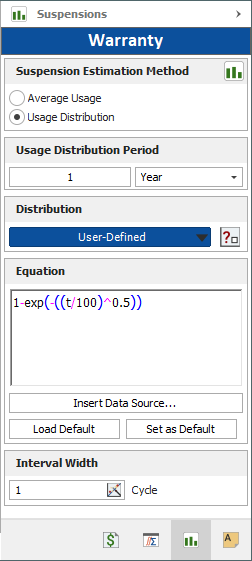
  • If you choose the User-Defined distribution, you can manually enter any equation that describes how customers use your product. You will need to use the variable t to represent time or usage, as in the example shown next.

You can also use distributions calculated in life data folios from your current project as data sources for your equation. To insert a data source, click the Insert Data Source button and select a calculated life data folio. The software will enter that source into the Equation area. You can insert multiple data sources and combine them (with operators such as + and *) to form new distributions.

To save the equation, click the Set as Default button. To automatically re-enter the saved equation in the Equations area, click Load Default.

• You will also be required to enter the Interval Width. This value is used to divide the usage distribution pdf into segments so the software can obtain the probability that any given unit will have accumulated usage at the rate represented by that segment. For example, if the usage distribution represents the number of pages printed per year and you enter 500 for the interval, the software will break the distribution into segments of 0 to 500 pages per year, 501 to 1000 pages per year, 1001 to 1500 pages per year, and so on.

The appropriate value for this field will depend upon your knowledge of typical product usage levels. The interval width should be selected such that when the warranty data are converted into failure/suspension times, the resulting times-to-suspension will neither be too close together (too few suspension units per interval) or too far apart (too many suspension units per interval). If you find that the failure/suspension data set is not acceptable, you can adjust the interval width and perform the calculation again. To help eliminate some of the guesswork, you can also use the Interval Width Estimator, which provides an approximation of the interval width based on the number of intervals and suspensions you specify. You can access the tool by clicking the icon in the Interval Width area of the control panel.

• When you click the Calculate icon on the Main page of the control panel, Weibull++ will perform the following calculations for each group of units that have the same date in-service:
  1. Calculate the number of units from the sales group that were still operating at the end of the observation period:
     
     Number of Units Sold – Number of Units Returned = Number of Suspensions
  2. Calculate the amount of time (in days) that those units had been in service by the end of the observation period:
     
     End of Observation Period date – Date In-Service = Days in Service
  3. Use the Interval Width to split the usage distribution into segments and calculate the probability that any given unit will fall into each segment:
     
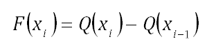
     where Q( ) is the cumulative distribution function (cdf) of the usage distribution and x represents the intervals used in apportioning the suspensions.
  4. For each segment, calculate the number of suspensions that are expected to have accumulated usage at the rate represented by that segment. (Note that the software applies a correction factor in order to get a whole number of units for each interval.)
     
     Number of Suspensions x Percentage for the Segment
  5. If necessary, convert the usage value from the end of each segment to the daily rate for calculation purposes (e.g., if the segment represents users who typically print 201 - 400 pages per month, then the daily rate would be 400/30 or approximately 13.333 pages per day).
  6. For each segment, estimate the amount of usage the suspensions may have accumulated by the end of the observation period:
     
     Days in Service * Usage per Day = Estimated Usage at Time of Suspension

For example, suppose that the Sales sheet records that 100 printers entered service on January 1st while the Returns sheet records the number of pages printed for the 20 units from this sales group that have been returned. If you enter December 31st for the End of Observation Period date and the usage distribution indicates that 25% of users are likely to print 50 -100 pages per month, the software will calculate the usage for this segment of the January 1st sales group as follows:

• 100 Units Sold – 20 Units Returned = 80 Suspensions
• December 31st – January 1st = 365 Days in Service
• 80 Suspensions x 25% = 20 Units printing 50 - 100 pages per month (or ~3.33 pages per day)
• 365 Days in Service * 3.33 Pages per Day = 1215.45 Pages approximately

When you click the Show Analysis Summary button on the Main page of the control panel, the life data analysis data set will include one row with 20 suspensions at "End Time" = 1215.45. There will be additional rows for the remaining 60 suspensions from the January 1st sales group, which will reflect the different usage amounts calculated based on the other segments of the usage distribution.