Dynamic Overlaid Contour Plot
The dynamic overlaid contour plot displays a series of overlaid contour plots side by side. The x- and y-axes represent two of the quantitative factors. The level of one or more additional factors is varied across the plots. This plot is available for all designs with at least three factors, where at least two of the factors are quantitative.
Creating the Dynamic Overlaid Contour Plot
There are two ways to create a dynamic overlaid contour plot:
- On the Home tab, click the Optimization icon in the Insert gallery.
![]()
In the Select Optimization Tool window that appears, select a folio to optimize and then select to create a dynamic overlaid contour plot.
- Open an existing optimization folio and add additional optimization tools based on the same design folio by choosing Optimization > Tools > Add Optimization Tool.
Note that each optimization folio can have only one optimization tool of each type.
When you first create a dynamic overlaid contour plot, you will need to specify the settings that the plot is based on. The Dynamic Overlaid Contour Plot Settings window will appear automatically. The navigation panel on the left of this windows lists all of the settings pages.
The pages listed under the Responses heading allow you to select which response(s) you want to optimize, and to specify the optimal settings for each response.
Click each response under the Responses heading and use the Include in optimization drop-down to specify whether the response will be optimized.
Then use the Goal field to specify whether you want to minimize the response, maximize it or get it within a range of values. You will then specify a lower limit and/or an upper limit for the response, depending on which action you have selected.
Note that if a transformation has been applied to any response that you are optimizing, the transformed response values are used in optimization. For this reason, the values that you enter for Lower Limit and/or Upper Limit must also be transformed values. For example, life data responses always have the lognormal transformation applied; therefore, if you are maximizing a life data response, the Lower Limit value should be in terms of Ln(failure time).
The pages listed under the Factor heading allows you to specify which factors will be shown on the x- and y-axes and whether to vary or hold constant each factor not shown on the axes, as well as the value ranges to use for the factors. The factor values are expressed in terms of actual or coded values. To change the setting, close the Optimization Settings window and choose Plot > Display > [Value Type].
Click each factor and use the Treatment in Plot field to specify how it should be used in the plot. You should set one quantitative factor to be displayed on the x-axis and another quantitative factor to be displayed on the y-axis. The remaining factors may each be either held constant or varied.
For factors displayed on the axes, use the Lower Limit and Upper Limit fields to specify the bounds for each factor.
For factors that are held constant, specify the setting used for the factor in the Constant Value field. If the factor is qualitative, a drop-down list of the available factor settings will be provided.
For quantitative factors that are varied, use the Lower Limit and Upper Limit fields to specify the bounds for each factor. Then enter the number of different settings within that range to use for the factor in the Number of Intervals field. Qualitative factors will be varied across all possible settings. Note that if a response is missing all data at a given level for a qualitative factor or a block (which is essentially a type of qualitative factor), that level cannot be included in the optimization of the response. Therefore, any level that does not have data for a given response will instead be treated as equal to 0 in the optimization of that response.
The settings that you specify for the factors that are varied determine the number of possible solutions (i.e., plots) that will be generated and evaluated to determine if they contain a feasible region.
The Summary page allows you to review all your optimization settings.
Once you have specified and reviewed the settings, click OK. The dynamic overlaid contour plot will be created. As the range of solutions are examined, the plots for the solutions are displayed. Once all solutions have been considered, the first overlaid contour plot is displayed. Additional solutions will be displayed in the Sorted Solutions area on the control panel.
Note:
You can specify new settings at any time by clicking the Calculate icon ( ![]() ) to re-open the Dynamic
Overlaid Contour Plot Settings window. You can also change the
folio that the dynamic overlaid contour plot is based on by clicking
the Select Data Source
icon (
) to re-open the Dynamic
Overlaid Contour Plot Settings window. You can also change the
folio that the dynamic overlaid contour plot is based on by clicking
the Select Data Source
icon ( ![]() ).
).
Viewing the Dynamic Overlaid Contour Plot
When the dynamic overlaid contour plot is created, all of the factor setting combinations that are possible based on your settings in the Dynamic Overlaid Contour Plot Settings window are generated and examined to determine whether they contain a feasible region (i.e., a region where response values fall within the specified range). All factor setting combinations that contain a feasible region are listed in the Sorted Solutions area on the control panel. You can select multiple solutions to be displayed side by side; up to 99 overlaid contour plots can be displayed simultaneously.
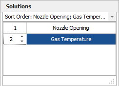
To facilitate finding and displaying solutions of interest to you, the order in which the solutions are sorted can be changed. Click the drop-down in the Solutions area to view a list of the factors that are either varied or held constant. Use the Priority Up and Priority Down arrows that appear when you click a priority number in the first column to move the factors up and down the list. In the example shown next, the solutions are being sorted first by the Nozzle Opening factor setting, then by the Gas Temperature factor setting.
This results in the following sorted list, where solutions are sorted by Gas Temperature within Nozzle Opening settings:
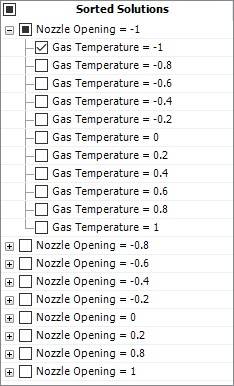
You can then select or clear entire groups of solutions for display.