
Duane Model
In 1962, J. T. Duane published a report in which he presented failure data of different systems during their development programs [8]. While analyzing the data, it was observed that the cumulative MTBF versus cumulative operating time followed a straight line when plotted on log-log paper, as shown next.
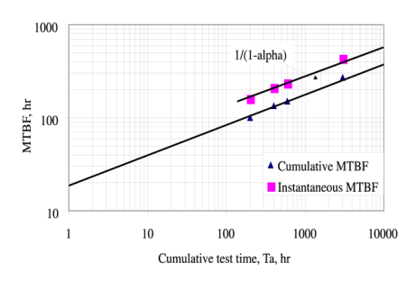
Based on that observation, Duane developed his model as follows. If
 is the number of failures by time
 , the observed mean (average) time between failures,
 at time
 is:
is:


The equation of the line can be expressed as:


Setting:


yields:


Then equating  to its expected value, and assuming an exact linear relationship, gives:


or:


And, if you assume a constant failure intensity, then the cumulative failure intensity,
 , is:
, is:


or:


Also, the expected number of failures up to time
 is:
is:


where:
 is the average estimate of the cumulative failure intensity, failures/hour.
 is the total accumulated unit hours of test and/or development time.
 is the cumulative failure intensity at
 or at the beginning of the test, or the earliest time at which the first
 is predicted, or the
 for the equipment at the start of the design and development process.
 is the improvement rate in the
 .
.


The corresponding  , or
, or
 , is equal to:


where  cumulative MTBF at
 or at the beginning of the test, or the earliest time at which the first
 can be determined, or the
 predicted at the start of the design and development process (
 ).
).


The cumulative MTBF,  , and
, and
 tell whether
 is increasing or
 is decreasing with time, utilizing all data up to that time. You may want to know, however, the instantaneous
 or
or
 to see what you are doing at a specific instant or after a specific test and development time. The instantaneous failure intensity,
 , is:
, is:


Similarly, using the equation for the expected number of failures up to time
 , this procedure yields:


where  implies infinite MTBF growth.

As shown in these derivations, the instantaneous failure intensity improvement line is obtained by shifting the cumulative failure intensity line down, parallel to itself, by a distance of
 . Similarly, the current or instantaneous MTBF growth line is obtained by shifting the cumulative MTBF line up, parallel to itself, by a distance of
 , as illustrated in the figure below.


Parameter Estimation
The Duane model is a two parameter model. Therefore, to use this model as a basis for predicting the reliability growth that could be expected in an equipment development program, procedures must be defined for estimating these parameters as a function of equipment characteristics. Note that, while these parameters can be estimated for a given data set using curve-fitting methods, there exists no underlying theory for the Duane model that could provide a basis for a priori estimation.
One of the parameters of the Duane model is
 . The second parameter can be represented as
 or
or
 where
where
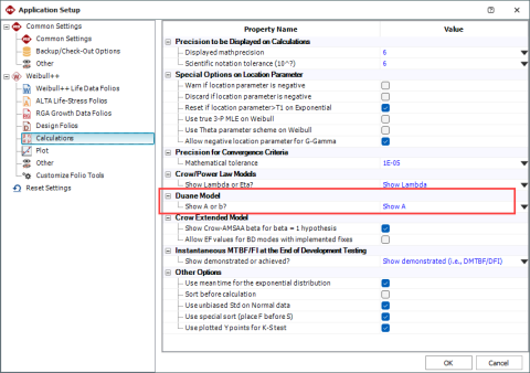
 . There is an option within the Application Setup that allows you to determine whether to display
 or
or
 for the Duane model. All formulation within this reference uses the parameter
 .
.


Graphical Method
The Duane model for the cumulative failure intensity is:

This equation may be linearized by taking the natural log of both sides:


Consequently, plotting  versus
 on log-log paper will result in a straight line with a negative slope, such that:
 is the y-intercept at

 is the cumulative failure intensity at

 is the slope of the straight line on the log-log plot


Similarly, the corresponding MTBF of the cumulative failure intensity can also be linearized by taking the natural log of both sides:


Plotting  versus
 on log-log paper will result in a straight line with a positive slope such that:
 is the y-intercept at

 is the cumulative mean time between failure at

 is the slope of the straight line on the log-log plot

Two ways of determining these curves are as follows:
1. Predict the  and
and

 of the system from its reliability block diagram and available component failure intensities. Plot this value on log-log plotting paper at
 From past experience and from past data for similar equipment, find values of
 , the slope of the improvement lines for
 or
or
 . Modify this
 as necessary. If a better design effort is expected and a more intensive research, test and development or TAAF program is to be implemented, then a 15% improvement in the growth rate may be attainable. Consequently, the available value for slope
 , and
, and
 , should be adjusted by this amount. The value to be used will then be
 A line is then drawn through point
 and
and
 with the just determined slope
 , keeping in mind that
 is negative for the
 curve. This line should be extended to the design, development and test time scheduled to be expended to see if the failure intensity goal will indeed be achieved on schedule. It is also possible to find that the design, development and test time to achieve the goal may be earlier than the delivery date or later. If earlier, then either the reliability program effort can be judiciously and appropriately trimmed; or if it is an incentive contract, full advantage is taken of the fact that the failure intensity goal can be exceeded with the associated increased profits to the company. A similar approach may be used for the MTBF growth model, where
 is plotted at
 , and a line is drawn through the point
 and
and
 with slope
 to obtain the MTBF growth line. If
 values are not available, consult the table below, which gives actual
 values for various types of equipment. These have been obtained from literature or by MTBF growth tests. It may be seen from the following table that
 values range between 0.24 and 0.65. The lower values reflect slow early growth and the higher values reflect fast early growth.


| Equipment | Slope( ) )
|
|
|---|---|---|
| Computer system | Actual | 0.24 |
| Easy to find failures were eliminated | 0.26 | |
| All known failure causes were eliminated | 0.36 | |
| Mainframe computer | 0.50 | |
| Aerospace electronics | All malfunctions | 0.57 |
| Relevant failures only | 0.65 | |
| Attack radar | 0.60 | |
| Rocket engine | 0.46 | |
| Afterburning turbojet | 0.35 | |
| Complex hydromechanical system | 0.60 | |
| Aircraft generator | 0.38 | |
| Modern dry turbojet | 0.48 |
2. During the design, development and test phase and at specific milestones, the
 is calculated from the total failures and
 values. These values of
 or
or
 are plotted above the corresponding
 values on log-log paper. A straight line is drawn favoring these points to minimize the distance between the points and the line, thus establishing the improvement or growth model and its parameters graphically. If needed, linear regression analysis techniques can be used to determine these parameters.

Graphical Method Example
A complex system's reliability growth is being monitored and the data set is given in the table below.
| Point Number | Cumulative Test Time (hours) | Cumulative Failures | Cumulative MTBF(hours) | Instantaneous MTBF (hours) |
|---|---|---|---|---|
| 1 | 200 | 2 | 100.0 | 100 |
| 2 | 400 | 3 | 133.0 | 200 |
| 3 | 600 | 4 | 150.0 | 200 |
| 4 | 3,000 | 11 | 273.0 | 342.8 |
Do the following:
- Plot the cumulative MTBF growth curve.
- Write the equation of this growth curve.
- Write the equation of the instantaneous MTBF growth model.
- Plot the instantaneous MTBF growth curve.
Solution
- Given the data in the second and third columns of the above table, the cumulative MTBF,
 , values are calculated in the fourth column. The information in the second and fourth columns are then plotted. The first figure below shows the cumulative MTBF while the second figure below shows the instantaneous MTBF. It can be seen that a straight line represents the MTBF growth very well on log-log scales.
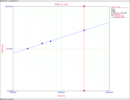
Cumulative MTBF plot 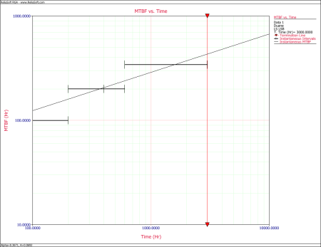
Instantaneous MTBF plot By changing the x-axis scaling, you are able to extend the line to
 . You can get the value of
 from the graph by positioning the cursor at the point where the line meets the y-axis. Then read the value of the y-coordinate position at the bottom left corner. In this case,
 is approximately 14 hours. The next figure illustrates this.
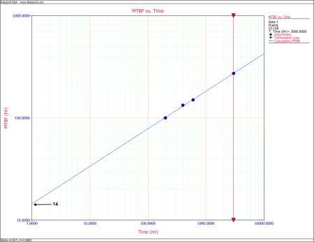
Cumulative MTBF plot for  at
at

Another way of determining
 is to calculate
 by using two points on the fitted straight line and substituting the corresponding
 and
and
 values into:
Then substitute this
 and choose a set of values for
 and
and
 into the cumulative MTBF equation,
 , and solve for
 . The slope of the line,
 , may also be found from the linearized form of the cumulative MTBF equation, or :
Using the cumulative MTBF plot for the example, at
 hours,
 hours, and
 hours,
 hours. From the cumulative MTBF plot for
 hours when
 , substituting the first set of values,
 hours and
 , into the equation yields:
- Substituting the second set of values,
 hours and
 into the equation yields:
 values yields a better estimate of
 .
.
- Now the equation for the cumulative MTBF growth curve is:
- Using the following equation for the instantaneous MTBF, or
 , line by a distance of
 gives the instantaneous MTBF, or the
 , line.
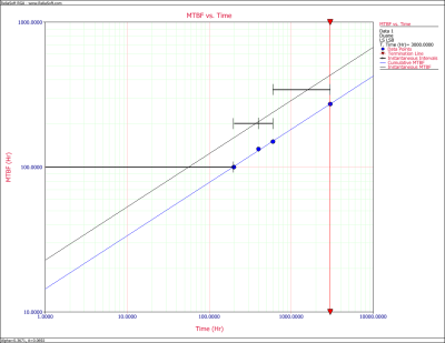
Cumulative and Instantaneous MTBF vs. Time plot


Least Squares (Linear Regression)
The parameters can also be estimated using a mathematical approach. To do this, linearize the MTBF of the cumulative failure intensity by taking the natural log of both sides, and then apply least squares analysis. For example:

For simplicity in the calculations, let:


Therefore, the equation becomes:


Assume that a set of data pairs  ,
,
 ,...,
,...,
 were obtained and plotted. Then according to the Least Squares Principle, which minimizes the vertical distance between the data points and the straight line fitted to the data, the best fitting straight line to this data set is the straight line
 such that:


where  and
and
 are the least squares estimates of
 and
and
 . To obtain
 and
and
 , let:


Differentiating  with respect to
 and
and
 yields:


and:


Set those two equations equal to zero:


and:


Solve the equations simultaneously:


and:


Now substituting back 

 and
and
 we have:


![{\displaystyle {\hat {b}}={{e}^{{\tfrac {1}{n}}\left[{\underset {i=1}{\overset {n}{\mathop {\sum } }}}\,\ln({{m}_{ci}})-\alpha {\underset {i=1}{\overset {n}{\mathop {\sum } }}}\,\ln({{T}_{i}})\right]}}\,\!}](https://en.wikipedia.org/api/rest_v1/media/math/render/svg/5e78ff7d8b9adeece332119421355de55fbfabf8)
where:

![{\displaystyle {\hat {\alpha }}={\frac {{\underset {i=1}{\overset {n}{\mathop {\sum } }}}\,\ln({{T}_{i}})\ln({{m}_{ci}})-{\tfrac {{\underset {i=1}{\overset {n}{\mathop {\sum } }}}\,\ln({{T}_{i}}){\underset {i=1}{\overset {n}{\mathop {\sum } }}}\,\ln({{m}_{ci}})}{n}}}{{\underset {i=1}{\overset {n}{\mathop {\sum } }}}\,{{\left[\ln({{T}_{i}})\right]}^{2}}-{\tfrac {{\left({\underset {i=1}{\overset {n}{\mathop {\sum } }}}\,\ln({{T}_{i}})\right)}^{2}}{n}}}}\,\!}](https://en.wikipedia.org/api/rest_v1/media/math/render/svg/962b1f979596d60cc018c990bee0d33230469054)
Example 1
Using the same data set from the graphical approach example, estimate the parameters of the MTBF model using least squares.
Solution
From the data table:

![{\displaystyle {\begin{aligned}{\underset {i=1}{\overset {n}{\mathop {\sum } }}}\,\ln({{T}_{i}})&=&25.693\\{\underset {i=1}{\overset {n}{\mathop {\sum } }}}\,\ln({{T}_{i}})\ln({{m}_{ci}})&=&130.66\\{\underset {i=1}{\overset {n}{\mathop {\sum } }}}\,\ln({{m}_{ci}})&=&20.116\\{\underset {i=1}{\overset {n}{\mathop {\sum } }}}\,{{\left[\ln({{T}_{i}})\right]}^{2}}&=&168.99\end{aligned}}\,\!}](https://en.wikipedia.org/api/rest_v1/media/math/render/svg/3866044eca65ee1c232a9993bba2dbb05171be1d)
Obtain the value of  from the least squares analysis, or:


![{\displaystyle {\begin{aligned}{\hat {\alpha }}&={\frac {{\underset {i=1}{\overset {n}{\mathop {\sum } }}}\,\ln({{T}_{i}})\ln({{m}_{ci}})-{\tfrac {{\underset {i=1}{\overset {n}{\mathop {\sum } }}}\,\ln({{T}_{i}}){\underset {i=1}{\overset {n}{\mathop {\sum } }}}\,\ln({{m}_{ci}})}{n}}}{{\underset {i=1}{\overset {n}{\mathop {\sum } }}}\,{{\left[\ln({{T}_{i}})\right]}^{2}}-{\tfrac {{\left({\underset {i=1}{\overset {n}{\mathop {\sum } }}}\,\ln({{T}_{i}})\right)}^{2}}{n}}}}\\&={\frac {130.66-{\tfrac {25.693\cdot 20.116}{4}}}{168.99-{\tfrac {{25.693}^{2}}{4}}}}\\&=0.3671\end{aligned}}\,\!}](https://en.wikipedia.org/api/rest_v1/media/math/render/svg/9977831b8a2d2dc1067e7be756dbba9b38a69780)
Obtain the value  from the least squares analysis, or:


![{\displaystyle {\begin{aligned}{\hat {b}}&={{e}^{{\tfrac {1}{n}}\left[{\underset {i=1}{\overset {n}{\mathop {\sum } }}}\,\ln({{m}_{ci}})-\alpha {\underset {i=1}{\overset {n}{\mathop {\sum } }}}\,\ln({{T}_{i}})\right]}}\\&={{e}^{{\tfrac {1}{4}}(20.116-0.3671\cdot 25.693)}}\\&=14.456\end{aligned}}\,\!}](https://en.wikipedia.org/api/rest_v1/media/math/render/svg/087610126aca42d5ca22c266b59afad92f7877d6)
Therefore, the cumulative MTBF becomes:


The equation for the instantaneous MTBF growth curve is:


Example 2
For the data given in columns 1 and 2 of the following table, estimate the Duane parameters using least squares.
| (1)Failure Number | (2)Failure Time (hours) | (3)
|
(4)
|
(5)
|
(6)
|
(7)
|
|---|---|---|---|---|---|---|
| 1 | 9.2 | 2.219 | 4.925 | 9.200 | 2.219 | 4.925 |
| 2 | 25 | 3.219 | 10.361 | 12.500 | 2.526 | 8.130 |
| 3 | 61.5 | 4.119 | 16.966 | 20.500 | 3.020 | 12.441 |
| 4 | 260 | 5.561 | 30.921 | 65.000 | 4.174 | 23.212 |
| 5 | 300 | 5.704 | 32.533 | 60.000 | 4.094 | 23.353 |
| 6 | 710 | 6.565 | 43.103 | 118.333 | 4.774 | 31.339 |
| 7 | 916 | 6.820 | 46.513 | 130.857 | 4.874 | 33.241 |
| 8 | 1010 | 6.918 | 47.855 | 126.250 | 4.838 | 33.470 |
| 9 | 1220 | 7.107 | 50.504 | 135.556 | 4.909 | 34.889 |
| 10 | 2530 | 7.836 | 61.402 | 253.000 | 5.533 | 43.359 |
| 11 | 3350 | 8.117 | 65.881 | 304.545 | 5.719 | 46.418 |
| 12 | 4200 | 8.343 | 69.603 | 350.000 | 5.858 | 48.872 |
| 13 | 4410 | 8.392 | 70.419 | 339.231 | 5.827 | 48.895 |
| 14 | 4990 | 8.515 | 72.508 | 356.429 | 5.876 | 50.036 |
| 15 | 5570 | 8.625 | 74.393 | 371.333 | 5.917 | 51.036 |
| 16 | 8310 | 9.025 | 81.455 | 519.375 | 6.253 | 56.431 |
| 17 | 8530 | 9.051 | 81.927 | 501.765 | 6.218 | 56.282 |
| 18 | 9200 | 9.127 | 83.301 | 511.111 | 6.237 | 56.921 |
| 19 | 10500 | 9.259 | 85.731 | 552.632 | 6.315 | 58.469 |
| 20 | 12100 | 9.401 | 88.378 | 605.000 | 6.405 | 60.215 |
| 21 | 13400 | 9.503 | 90.307 | 638.095 | 6.458 | 61.375 |
| 22 | 14600 | 9.589 | 91.945 | 663.636 | 6.498 | 62.305 |
| 23 | 22000 | 9.999 | 99.976 | 956.522 | 6.863 | 68.625 |
| Sum = | 173.013 | 1400.908 | 7600.870 | 121.406 | 974.242 |


Solution
To estimate the parameters using least squares, the values in columns 3, 4, 5, 6 and 7 are calculated. The cumulative MTBF,
 , is calculated by dividing the failure time by the failure number. The value of
 is:
is:


![{\displaystyle {\begin{aligned}{\hat {\alpha }}&={\frac {{\underset {i=1}{\overset {n}{\mathop {\sum } }}}\,\ln({{T}_{i}})\ln({{m}_{ci}})-{\tfrac {{\underset {i=1}{\overset {n}{\mathop {\sum } }}}\,\ln({{T}_{i}}){\underset {i=1}{\overset {n}{\mathop {\sum } }}}\,\ln({{m}_{ci}})}{n}}}{{\underset {i=1}{\overset {n}{\mathop {\sum } }}}\,{{\left[\ln({{T}_{i}})\right]}^{2}}-{\tfrac {{\left({\underset {i=1}{\overset {n}{\mathop {\sum } }}}\,\ln({{T}_{i}})\right)}^{2}}{n}}}}\\&={\frac {974.242-{\tfrac {173.013\cdot 121.406}{23}}}{1400.908-{\tfrac {{(173.013)}^{2}}{23}}}}\\&=0.6133\end{aligned}}\,\!}](https://en.wikipedia.org/api/rest_v1/media/math/render/svg/563f6a58a384d6eb577a13213a49f7f6eb0ab75c)
The estimator of  is estimated to be:

![{\displaystyle {\begin{aligned}{\hat {b}}&={{e}^{{\tfrac {1}{n}}\left[{\underset {i=1}{\overset {n}{\mathop {\sum } }}}\,\ln({{m}_{ci}})-\alpha {\underset {i=1}{\overset {n}{\mathop {\sum } }}}\,\ln({{T}_{i}})\right]}}\\&={{e}^{{\tfrac {1}{23}}(121.406-0.6133\cdot 173.013)}}\\&=1.9453\end{aligned}}\,\!}](https://en.wikipedia.org/api/rest_v1/media/math/render/svg/5984ad205d9459d770c00a3c2689f8f663e4d814)
Therefore, the cumulative MTBF becomes:


Using the equation for the instantaneous MTBF growth curve,


Example 3
For the data given in the following table, estimate the Duane parameters using least squares.
| Run Number | Failed Unit | Test Time 1 | Test Time 2 | Cumulative Time |
|---|---|---|---|---|
| 1 | 1 | 0.2 | 2.0 | 2.2 |
| 2 | 2 | 1.7 | 2.9 | 4.6 |
| 3 | 2 | 4.5 | 5.2 | 9.7 |
| 4 | 2 | 5.8 | 9.1 | 14.9 |
| 5 | 2 | 17.3 | 9.2 | 26.5 |
| 6 | 2 | 29.3 | 24.1 | 53.4 |
| 7 | 1 | 36.5 | 61.1 | 97.6 |
| 8 | 2 | 46.3 | 69.6 | 115.9 |
| 9 | 1 | 63.6 | 78.1 | 141.7 |
| 10 | 2 | 64.4 | 85.4 | 149.8 |
| 11 | 1 | 74.3 | 93.6 | 167.9 |
| 12 | 1 | 106.6 | 103 | 209.6 |
| 13 | 2 | 195.2 | 117 | 312.2 |
| 14 | 2 | 235.1 | 134.3 | 369.4 |
| 15 | 1 | 248.7 | 150.2 | 398.9 |
| 16 | 2 | 256.8 | 164.6 | 421.4 |
| 17 | 2 | 261.1 | 174.3 | 435.4 |
| 18 | 2 | 299.4 | 193.2 | 492.6 |
| 19 | 1 | 305.3 | 234.2 | 539.5 |
| 20 | 1 | 326.9 | 257.3 | 584.2 |
| 21 | 1 | 339.2 | 290.2 | 629.4 |
| 22 | 1 | 366.1 | 293.1 | 659.2 |
| 23 | 2 | 466.4 | 316.4 | 782.8 |
| 24 | 1 | 504 | 373.2 | 877.2 |
| 25 | 1 | 510 | 375.1 | 885.1 |
| 26 | 2 | 543.2 | 386.1 | 929.3 |
| 27 | 2 | 635.4 | 453.3 | 1088.7 |
| 28 | 1 | 641.2 | 485.8 | 1127 |
| 29 | 2 | 755.8 | 573.6 | 1329.4 |
Solution
The solution to this example follows the same procedure as the previous example. Therefore, from the table shown above:


For least squares, the value of  is:
is:

![{\displaystyle {\begin{aligned}{\hat {\alpha }}&={\frac {{\underset {i=1}{\overset {n}{\mathop {\sum } }}}\,\ln({{T}_{i}})\ln({{m}_{ci}})-{\tfrac {{\underset {i=1}{\overset {n}{\mathop {\sum } }}}\,\ln({{T}_{i}}){\underset {i=1}{\overset {n}{\mathop {\sum } }}}\,\ln({{m}_{ci}})}{n}}}{{\underset {i=1}{\overset {n}{\mathop {\sum } }}}\,{{\left[\ln({{T}_{i}})\right]}^{2}}-{\tfrac {{\left({\underset {i=1}{\overset {n}{\mathop {\sum } }}}\,\ln({{T}_{i}})\right)}^{2}}{n}}}}\\&={\frac {483.154-{\tfrac {154.151\cdot 82.884}{29}}}{902.592-{\tfrac {{(154.151)}^{2}}{29}}}}\\&=0.5115\end{aligned}}\,\!}](https://en.wikipedia.org/api/rest_v1/media/math/render/svg/ef0c32f70b4d039551b5dd0f1ec1209204526e6e)
The value of the estimator  is:
is:

![{\displaystyle {\begin{aligned}{\hat {b}}&={{e}^{{\tfrac {1}{n}}\left[{\underset {i=1}{\overset {n}{\mathop {\sum } }}}\,\ln({{m}_{ci}})-\alpha {\underset {i=1}{\overset {n}{\mathop {\sum } }}}\,\ln({{T}_{i}})\right]}}\\&={{e}^{{\tfrac {1}{29}}(82.884-0.5115\cdot 154.151)}}\\&=1.1495\end{aligned}}\,\!}](https://en.wikipedia.org/api/rest_v1/media/math/render/svg/c55c86c0df5a508af3bfabdaa1c3565e7b2d5848)
Therefore, the cumulative MTBF is:


Using the equation for the instantaneous MTBF growth,


Maximum Likelihood Estimators
L. H. Crow [17] noted that the Duane model could be stochastically represented as a Weibull process, allowing for statistical procedures to be used in the application of this model in reliability growth. This statistical extension became what is known as the Crow-AMSAA (NHPP) model. The Crow-AMSAA model, which is described in the Crow-AMSAA (NHPP) chapter, provides a complete Maximum Likelihood Estimation (MLE) solution to the Duane model.
Confidence Bounds
Least squares confidence bounds can be computed for both the model parameters and metrics of interest for the Duane model.
Parameter Bounds
Apply least squares analysis on the Duane model:


The unbiased estimator of  can be obtained from:


![{\displaystyle {{\sigma }^{2}}=Var\left[\ln {{m}_{c}}(t)\right]={\frac {SSE}{(n-2)}}\,\!}](https://en.wikipedia.org/api/rest_v1/media/math/render/svg/d7cf655536f10ff2deae0bfa2469f50b1f45ccdb)
where:

![{\displaystyle SSE={\underset {i=1}{\overset {n}{\mathop {\sum } }}}\,{{\left[\ln {{\hat {m}}_{c}}({{t}_{i}})-\ln {{m}_{c}}({{t}_{i}})\right]}^{2}}\,\!}](https://en.wikipedia.org/api/rest_v1/media/math/render/svg/89e68bb9a64ed8161fdd0fb59e0e6bd18db82866)
Thus, the confidence bounds on  and
and
 are:
are:


![{\displaystyle C{{B}_{b}}={\hat {b}}{{e}^{\pm {{t}_{n-2,\alpha /2}}SE\left[\ln({\hat {b}})\right]}}\,\!}](https://en.wikipedia.org/api/rest_v1/media/math/render/svg/f29b157f0b9b2c99da47514bb68a1ec789a7ec72)
where  denotes the percentage point of the
 distribution with
 degrees of freedom such that
 and:
and:


![{\displaystyle SE\left[\ln({\hat {b}})\right]=\sigma \cdot {\sqrt {\frac {{\underset {i=1}{\overset {n}{\mathop {\sum } }}}\,{{(\ln {{t}_{i}})}^{2}}}{n\cdot {{S}_{xx}}}}}\,\!}](https://en.wikipedia.org/api/rest_v1/media/math/render/svg/e26a315055dd2a9eeeea401d2eaf501765e7162f)

![{\displaystyle {{S}_{xx}}=\left[{\underset {i=1}{\overset {n}{\mathop {\sum } }}}\,{{(\ln {{t}_{i}})}^{2}}\right]-{\frac {1}{n}}{{\left({\underset {i=1}{\overset {n}{\mathop {\sum } }}}\,\ln({{t}_{i}})\right)}^{2}}\,\!}](https://en.wikipedia.org/api/rest_v1/media/math/render/svg/2349a581351371bdc15e123d3e6d5054754fe277)
Other Bounds
Confidence bounds also can be obtained on the cumulative MTBF and the cumulative failure intensity:

![{\displaystyle C{{B}_{{m}_{c}}}={{\hat {m}}_{c}}(t){{e}^{\pm {{z}_{\alpha }}{\sqrt {Var\left[\ln({{\hat {m}}_{c}})\right]}}}}\,\!}](https://en.wikipedia.org/api/rest_v1/media/math/render/svg/8ef6d6dfeabddfb9fb32cacdf621317e1c935463)

![{\displaystyle Var\left[\ln({{\hat {m}}_{c}})\right]={\frac {\sum \limits _{i=1}^{n}{{\left(\ln {{\hat {m}}_{c}}({{t}_{i}})-\ln {{m}_{c}}({{t}_{i}})\right)}^{2}}}{n-2}}\cdot \left({\frac {1}{n}}+{\frac {{\left(\ln(t)-{\frac {\sum \limits _{i=1}^{n}{\ln({{t}_{i}})}}{n}}\right)}^{2}}{\sum \limits _{i=1}^{n}{{\left(\ln({{t}_{i}})-{\frac {\sum \limits _{i=1}^{n}{\ln({{t}_{i}})}}{n}}\right)}^{2}}}}\right)\,\!}](https://en.wikipedia.org/api/rest_v1/media/math/render/svg/e49e28a685f82a98cd5ae22d1f41efed261cc6c0)

![{\displaystyle {\begin{aligned}{{[{{\lambda }_{c}}(t)]}_{L}}=&{\frac {1}{{[{{m}_{c}}(t)]}_{u}}}\\{{[{{\lambda }_{c}}(t)]}_{U}}=&{\frac {1}{{[{{m}_{c}}(t)]}_{l}}}\end{aligned}}\,\!}](https://en.wikipedia.org/api/rest_v1/media/math/render/svg/ed5830d273a1f43f4a4f259e90d1ab4822fd3fdc)
When  is large, the approximate
 confidence bounds for instantaneous MTBF are given by:


![{\displaystyle {\begin{aligned}{{m}_{i}}{{(t)}_{L}}=&{\frac {{[{{m}_{c}}(t)]}_{L}}{\hat {\beta }}}\\{{m}_{i}}{{(t)}_{U}}=&{\frac {{[{{m}_{c}}(t)]}_{U}}{\hat {\beta }}}\end{aligned}}\,\!}](https://en.wikipedia.org/api/rest_v1/media/math/render/svg/d4b980fc39dbe2136bfdf904d3ffcfd3a5604d3c)
and


therefore, the confidence bounds on the instantaneous failure intensity are:

![{\displaystyle {\begin{aligned}{{[{{\lambda }_{i}}(t)]}_{L}}=&{\frac {1}{{[{{m}_{i}}(t)]}_{U}}}\\{{[{{\lambda }_{c}}(t)]}_{U}}=&{\frac {1}{{[{{m}_{i}}(t)]}_{L}}}\end{aligned}}\,\!}](https://en.wikipedia.org/api/rest_v1/media/math/render/svg/cd50148a7ab3673641166a9bcbbed8866c0cc48c)
Duane Confidence Bounds Example
Using the values of  and
and
 estimated from the least squares analysis in Least Squares Example 2:


Calculate the 90% confidence bounds for the following:
- The parameters
 and
and
 .
. - The cumulative and instantaneous failure intensity.
- The cumulative and instantaneous MTBF.
Solution
- Use the values of
 and
and
 estimated from the least squares analysis. Then:
 are:
are:
 are:
are:
- The cumulative failure intensity is:
 hours, the confidence bounds on cumulative failure intensity are:


- The cumulative MTBF is:
 hours, the confidence bounds on the cumulative MTBF are:

The next figure displays the instantaneous MTBF. Both are plotted with confidence bounds.


![{\displaystyle {\begin{aligned}{{S}_{xx}}&=\left[{\underset {i=1}{\overset {n}{\mathop {\sum } }}}\,{{(\ln {{t}_{i}})}^{2}}\right]-{\frac {1}{n}}{{\left({\underset {i=1}{\overset {n}{\mathop {\sum } }}}\,\ln({{t}_{i}})\right)}^{2}}\\&=1400.9084-1301.4545\\&=99.4539\end{aligned}}\,\!}](https://en.wikipedia.org/api/rest_v1/media/math/render/svg/82ddc8ef0c8e223c8550a835165164ea74f61a01)


![{\displaystyle {\begin{aligned}{{[{{\lambda }_{c}}(t)]}_{L}}=&0.00106780\\{{[{{\lambda }_{c}}(t)]}_{U}}=&0.00116825\end{aligned}}\,\!}](https://en.wikipedia.org/api/rest_v1/media/math/render/svg/cf3ca44a1c655d96b0834696c8fbb73aa693b5c7)

![{\displaystyle {\begin{aligned}{{[{{\lambda }_{i}}(t)]}_{L}}=&0.00041299\\{{[{{\lambda }_{c}}(t)]}_{U}}=&0.00045184\end{aligned}}\,\!}](https://en.wikipedia.org/api/rest_v1/media/math/render/svg/422a1f29882f7d053a38099c324ee1e6d398fc05)


More Examples
Estimating the Time Required to Meet an MTBF Goal
A prototype of a system was tested with design changes incorporated during the test. A total of 12 failures occurred. The data set is given in the following table.
| Failure Number | Cumulative Test Time (hours) |
|---|---|
| 1 | 80 |
| 2 | 175 |
| 3 | 265 |
| 4 | 400 |
| 5 | 590 |
| 6 | 1100 |
| 7 | 1650 |
| 8 | 2010 |
| 9 | 2400 |
| 10 | 3380 |
| 11 | 5100 |
| 12 | 6400 |
Do the following:
- Estimate the Duane parameters.
- Plot the cumulative and instantaneous MTBF curves.
- How many cumulative test and development hours are required to meet an instantaneous MTBF goal of 500 hours?
- How many cumulative test and development hours are required to meet a cumulative MTBF goal of 500 hours?
Solution
- The next figure shows the data entered into Weibull++ along with the estimated Duane parameters.

- The following figure shows the cumulative and instantaneous MTBF curves.

- The next figure shows the cumulative test and development hours needed for an instantaneous MTBF goal of 500 hours.

- The figure below shows the cumulative test and development hours needed for a cumulative MTBF goal of 500 hours.

Multiple Systems - Known Operating Times Example
Two identical systems were tested. Any design changes made to improve the reliability of these systems were incorporated into both systems when any system failed. A total of 29 failures occurred. The data set is given in the table below.
Do the following:
- Estimate the Duane parameters.
- Assume both units are tested for an additional 100 hours each. How many failures do you expect in that period?
- If testing/development were halted at this point, what would the reliability equation for this system be?
| Failure Number | Failed Unit | Test Time Unit 1 (hours) | Test Time Unit 2 (hours) |
|---|---|---|---|
| 1 | 1 | 0.2 | 2.0 |
| 2 | 2 | 1.7 | 2.9 |
| 3 | 2 | 4.5 | 5.2 |
| 4 | 2 | 5.8 | 9.1 |
| 5 | 2 | 17.3 | 9.2 |
| 6 | 2 | 29.3 | 24.1 |
| 7 | 1 | 36.5 | 61.1 |
| 8 | 2 | 46.3 | 69.6 |
| 9 | 1 | 63.6 | 78.1 |
| 10 | 2 | 64.4 | 85.4 |
| 11 | 1 | 74.3 | 93.6 |
| 12 | 1 | 106.6 | 103 |
| 13 | 2 | 195.2 | 117 |
| 14 | 2 | 235.1 | 134.3 |
| 15 | 1 | 248.7 | 150.2 |
| 16 | 2 | 256.8 | 164.6 |
| 17 | 2 | 261.1 | 174.3 |
| 18 | 2 | 299.4 | 193.2 |
| 19 | 1 | 305.3 | 234.2 |
| 20 | 1 | 326.9 | 257.3 |
| 21 | 1 | 339.2 | 290.2 |
| 22 | 1 | 366.1 | 293.1 |
| 23 | 2 | 466.4 | 316.4 |
| 24 | 1 | 504 | 373.2 |
| 25 | 1 | 510 | 375.1 |
| 26 | 2 | 543.2 | 386.1 |
| 27 | 2 | 635.4 | 453.3 |
| 28 | 1 | 641.2 | 485.8 |
| 29 | 2 | 755.8 | 573.6 |
Solution
- The figure below shows the data entered into Weibull++ along with the estimated Duane parameters.

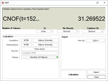
- The current accumulated test time for both units is 1329.4 hours. If the process were to continue for an additional combined time of 200 hours, the expected cumulative number of failures at
 is 31.2695, as shown in the figure below. At T = 1329.4, the expected number of failures is 29.2004. Therefore, the expected number of failures that would be observed over the additional 200 hours is
 .
.
- If testing/development were halted at this point, the system failure intensity would be equal to the instantaneous failure intensity at that time, or
 failures/hour. See the following figure.
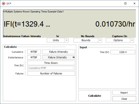
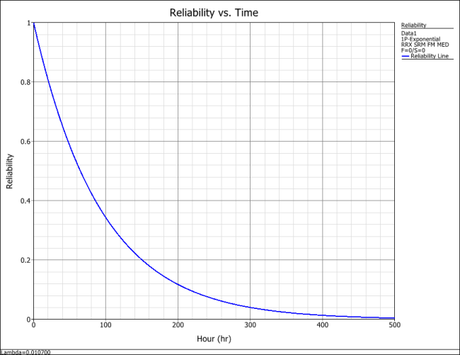
An exponential distribution can be assumed since the value of the failure intensity at that instant in time is known. Therefore:
Weibull++ can be utilized to provide a Reliability vs. Time plot which is shown below.


Using the Duane Model for Success/Failure Data
Given the sequential success/failure data in the table below, do the following:
- Estimate the Duane parameters.
- What is the instantaneous Reliability at the end of the test?
- How many additional test runs with a one-sided 90% confidence level are required to meet an instantaneous Reliability goal of 80%?
| Run Number | Result |
|---|---|
| 1 | F |
| 2 | F |
| 3 | S |
| 4 | S |
| 5 | S |
| 6 | F |
| 7 | S |
| 8 | F |
| 9 | F |
| 10 | S |
| 11 | S |
| 12 | S |
| 13 | F |
| 14 | S |
| 15 | S |
| 16 | S |
| 17 | S |
| 18 | S |
| 19 | S |
| 20 | S |
Solution
- The following figure shows the data set entered into Weibull++ along with the estimated Duane parameters.
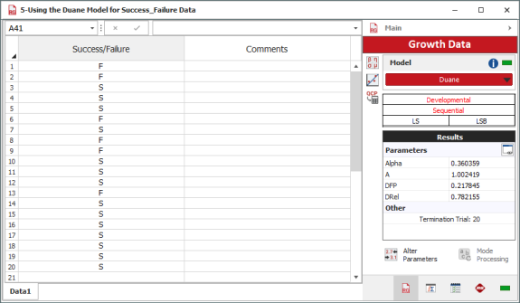
- The Reliability at the end of the test is equal to 78.22%. Note that this is the DRel that is shown in the control panel in the above figure.
- The figure below shows the number of test runs with both one-sided confidence bounds at 90% confidence level to achieve an instantaneous Reliability of 80%. Therefore, the number of additional test runs required with a 90% confidence level is equal to
 test runs.

