Discrete Reliability Growth Planning
To be consistent with the Duane postulate and the Crow (AMSAA) model, the discovery function must be of the same form. This form of the discovery function is an important property of the Crow Extended model and Crow Extended Discrete Planning model. As with the Crow (AMSAA) model, this form of the discovery function ties the model directly to real-world data and experiences. Therefore, a desirable feature of a discrete reliability growth planning model is that expected number of distinct failure modes over
. This implies that the probability,
, of a new distinct failure mode occurring at trial
is given by:
Let be the Type A initial failure probability and let
be the Type B initial failure probability.
A system failure occurs at the first event of a Type A mode or a Type B mode. Only one event causes a system failure. That is, Type A failures and Type B failures are disjointed.
The initial system failure probability
is:
The Type A failure probability is the failure probability in that part of the system that will not be addressed by corrective actions even if a failure mode is seen during test. The Type B failure probability is the failure probability in that part of the system that will be addressed by corrective actions if a failure mode is seen during test.
When a failure mode in the Type B part of the system is seen during test, a corrective action will be implemented. For discrete trials, the corrective action is always implemented at a later time after the failure mode is first seen.
When a corrective action is implemented for a Type B failure mode, the failure probability for that mode is reduced if the corrective action is effective. The fraction decrease in the Type B failure modes due to corrective actions is
, where the Average Effectiveness Factor (EF) is
and the corrective action may be implemented before the next trial or at a later date.
The management strategy ratio is:
The is the fraction of the initial system failure probability that will be addressed by corrective actions, if seen during the test.
If all Type B failure modes are seen and corrected with an average EF
, then the maximum reduction in the initial system failure probability is the Growth Potential failure probability:
The initial system Mean Trials Between Failure (MTrBF) is:
The Growth Potential MTrBF is:
Nominal Idealized Growth Curve
The nominal idealized growth curve portrays a general profile for reliability growth throughout system testing. It represents a best case scenario where fix delay is not taken into account.
The Crow Extended Discrete Planning Model Nominal Idealized Growth Curve failure probability as a function of test trials
is:
where is the initialization time, and
is the number of test trials.
It is virtually impossible to justify with any model that reliability growth starts at time zero because growth can only start when a Type B failure mode occurs. The Extended Discrete Planning Model Nominal Idealized Growth Curve failure probability is initially set equal to the initial failure probability
until the time
when:
The Initialization time allows for the probability of a Type B failure mode to be greater than zero before growth starts.
is then solved numerically.
The mean time to the first failure mode is given by the mean of a sequence of independent Bernoulli Trials, each trial with a different probability of a new failure mode given by:
Then the mean trial to the first Type B mode is given by:
where:
is then solved numerically.
Nominal Time to Reach Goal
The nominal time to reach the goal is calculated by setting the nominal idealized failure intensity,
, equal to the failure intensity goal,
. Therefore,
is solved numerically.
Actual Idealized Growth Curve
The Actual Idealized Growth Curve is a continuous function that incorporates the test phase average fix delay times and goes through each of the test phase target MTrBF.
Fix Delay
The fix delay reflects how long it takes from the time a problem failure mode is discovered in test to the time the corrective action is incorporated into the system and reliability growth is realized. The consideration of the fix delay is often in terms of how much calendar time it takes to incorporate a corrective action fix after the problem is first seem. However, the impact of the fix delay on reliability growth is reflected in the average test time it takes between finding a problem failure mode and incorporating a corrective action.
There can be a constant fix delay across all test phases or, as a practical matter, each test phase can have a different fix delay time. In practice, the fix delay will be considered constant over a test phase.
denotes the fix delay for phase
where
is the total number of phases in the test. The Weibull++ software allows for a maximum of ten test phases.
Actual Failure Intensity Function
Test Phase 1
The actual failure intensity function for test phase 1 is given by:
Note that the end time of Phase 1, must be greater than
. That is,
.
The actual idealized curve initialization time for Phase 1,
, is calculated from:
By obtaining the initial failure intensity for
:
Test Phase i
For any test phase , the actual idealized curve failure intensity is given by:
where and
is the test time of each corresponding test phase.
Actual Time to Reach Goal
The actual time to reach the goal is calculated using the actual failure intensity equation by solving for
such that the
is equal to the failure intensity goal,
. Therefore:
.
is solved numerically where
and
correspond to the phase in which the goal is met.
If the goal, , is met after the final test phase, then the actual time to reach the goal is not calculated since additional phases have to be added with specific duration and fix delays. The reliability growth program can be re-evaluated with the following options:
- Add more phase(s) to the program.
- Re-examine the phase duration of the existing phases.
- Investigate whether there are potential process improvements in the program that can reduce the average fix delay for the phases.
Other alternative routes for consideration would be to investigate the rest of the inputs in the model:
- Change the management strategy.
- Consider if further program risk can be acceptable, and if so, reduce the growth potential design margin.
- Consider if it is feasible to increase the effectiveness factors of the delayed fixes by using more robust engineering redesign methods.
Note that each change of input variables into the model can significantly influence the results.
With that in mind, any alteration in the input parameters should be justified by actionable decisions that will influence the reliability growth program. For example, increasing the average effectiveness factor value should be done only when there is proof that the program will pursue a different, more effective path in terms of addressing fixes.
Example
A missile system will be going through a reliability growth development program. The goal for the system is to reach a reliability requirement of 0.9 at the end of the program. This corresponds to a goal MTrBF,
, of 10 trials. The new missile system is similar to an existing missile system, but this will not be an upgrade. Therefore, to help design the reliability growth plan for the new system, parameters from the existing version will be used.
The previous missile system met its reliability goal of
which corresponds to a MTrBF = 20. There were over 600 trials of this missile system during developmental testing. The trials were used for testing and training. In addition, given the complexity of the technology that was utilized, additional trials were needed. The system also had an initial reliability of
. Additional parameters associated with the previous system are given below:
- Average Effectiveness Factor is
- Discovery Beta is
- Management Strategy Ratio is
- Growth Potential Design Margin is
For the new program, a will be used, along with an average
. For initial planning purposes, the average fix delay will be assumed to be equal to zero. Therefore, the nominal idealized curve will equal the actual idealized curve.
Determine the following:
- The growth potential MTrBF and failure intensity.
- The initial failure intensity and reliability.
- The growth potential reliability.
- The type A and type B initial failure intensity.
- The parameter
of the Crow extended model.
- The type B failure mode discovery function.
- The initialization time,
for the nominal failure intensity function.
- The nominal idealized failure intensity function.
- The nominal time to reach the MTrBF goal.
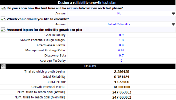
- Use Weibull++ to generate the reliability growth plan for the new missile design.
Solution
- The growth potential MTrBF is:
- The growth potential failure intensity is equal to:
- The growth potential reliability is equal to:
- The type A failure mode intensity,
is:
is:
- The initial MTrBF is:
is estimated such that:
- The type B failure mode discovery function is:
and
are known:
- The initialization time,
is calculated using the nominal idealized equation and setting this equal to initial failure intensity.
- The nominal idealized growth curve is given by the following equation:
- The nominal time to reach the MTrBF goal is estimated by solving for the value of
such that the nominal idealized curve
is equal to
. Therefore, solve for
such that:
trials.
- The reliability growth plan in Weibull++ is shown next.

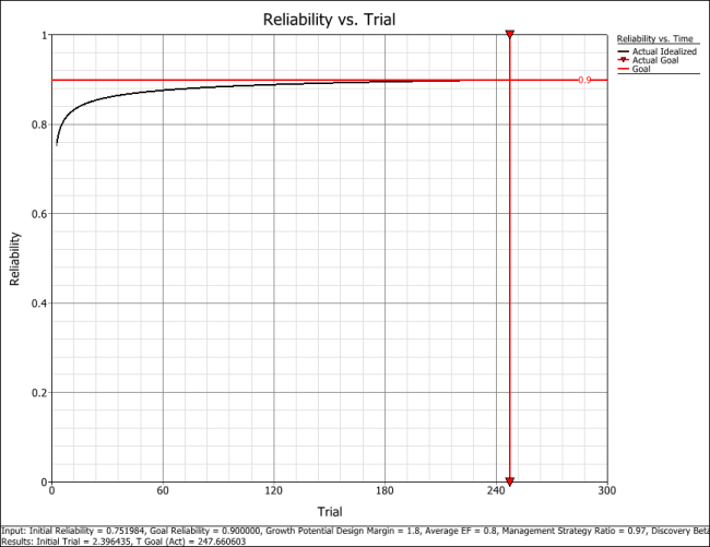
The plot of the reliability growth plan is shown below.


![{\displaystyle {{f}_{NI}}(t)={{f}_{A}}+(1-d){{f}_{B}}+d\left[\lambda {{t}^{\beta }}-\lambda {{(t-1)}^{\beta }}\right]{\text{ for }}t\geq {{t}_{0}}\,\!}](https://en.wikipedia.org/api/rest_v1/media/math/render/svg/76d74a2aa8cffccf74440fd75e8192ec7215645b)


![{\displaystyle {{f}_{NI}}({{t}_{0}})={{f}_{A}}+(1-d){{f}_{B}}+d\left[\lambda {{t}^{\beta }}-\lambda {{({{t}_{0}}-1)}^{\beta }}\right]={{f}_{I}}\,\!}](https://en.wikipedia.org/api/rest_v1/media/math/render/svg/e78ea2eb70c6d509f11d63e16043d622d5e0f98c)

![{\displaystyle MTrB{{F}_{B}}=\sum \limits _{k=1}^{\infty }{k\centerdot {{g}_{k}}}\centerdot \left[\prod \limits _{j=1}^{k-1}{{P}_{j}}\right]\,\!}](https://en.wikipedia.org/api/rest_v1/media/math/render/svg/9f371930aa3cf9b09bec85f4962c6305959a08a3)

![{\displaystyle {{g}_{k}}=\lambda \left[\mathop {k} ^{\beta }-{{\left(k-1\right)}^{\beta }}\right]\,\!}](https://en.wikipedia.org/api/rest_v1/media/math/render/svg/f30c5d5925b4db96a201a7661766e2c00da71308)


![{\displaystyle {{f}_{G}}={{f}_{A}}+(1-d){{f}_{B}}+d\left[\lambda {{t}_{N,G}}^{\beta }-\lambda {{\left({{t}_{N,G}}-1\right)}^{\beta }}\right]\,\!}](https://en.wikipedia.org/api/rest_v1/media/math/render/svg/91b6cf1e84b72fb7f958a5b36bb07bc045db7b5a)


![{\displaystyle {{f}_{AI}}(t)={{f}_{A}}+(1-d){{f}_{B}}+d\lambda \left[{{\left(\left({\frac {{{T}_{1}}-{{L}_{1}}}{{T}_{1}}}\right)t\right)}^{\beta }}-{{\left(\left({\frac {{{T}_{1}}-{{L}_{1}}}{{T}_{1}}}\right)t-1\right)}^{\beta }}\right]{\text{ for }}0<t\leq {{T}_{1}}\,\!}](https://en.wikipedia.org/api/rest_v1/media/math/render/svg/c4236641f84468db279fcf586e59929e7d0b201f)


![{\displaystyle {{f}_{AI}}(T_{0}^{AIC})={{\lambda }_{A}}+(1-d){{\lambda }_{B}}+d\lambda \left[{{\left(\left({\frac {{{T}_{1}}-{{L}_{1}}}{{T}_{1}}}\right)T_{0}^{AIC}\right)}^{\beta }}-{{\left(\left({\frac {{{T}_{1}}-{{L}_{1}}}{{T}_{1}}}\right)T_{0}^{AIC}-1\right)}^{\beta }}\right]\,\!}](https://en.wikipedia.org/api/rest_v1/media/math/render/svg/0dcbe7d8daf1dadacb724b6f39a66d888fa86b3e)


![{\displaystyle {{f}_{AI}}(t)={{f}_{A}}+(1-d){{f}_{B}}+d\lambda \left[{{\left({{T}_{i-1}}-{{L}_{i-1}}+\left({\frac {{{T}_{i}}-{{L}_{i}}-{{T}_{i-1}}+{{L}_{i-1}}}{{{T}_{i}}-{{T}_{i-1}}}}\right)(t-{{T}_{i-1}})\right)}^{\beta }}-{{\left({{T}_{i-1}}-{{L}_{i-1}}+\left({\frac {{{T}_{i}}-{{L}_{i}}-{{T}_{i-1}}+{{L}_{i-1}}}{{{T}_{i}}-{{T}_{i-1}}}}\right)(t-{{T}_{i-1}})-1\right)}^{\beta }}\right]\,\!}](https://en.wikipedia.org/api/rest_v1/media/math/render/svg/3751ada2fac59dcb89b4a6bd714ff1b56f38b148)


![{\displaystyle {{f}_{G}}={{f}_{A}}+(1-d){{f}_{B}}+d\lambda \left[{{\left({{T}_{i-1}}-{{L}_{i-1}}+\left({\frac {{{T}_{i}}-{{L}_{i}}-{{T}_{i-1}}+{{L}_{i-1}}}{{{T}_{i}}-{{T}_{i-1}}}}\right)({{t}_{AC,G}}-{{T}_{i-1}})\right)}^{\beta }}-{{\left({{T}_{i-1}}-{{L}_{i-1}}+\left({\frac {{{T}_{i}}-{{L}_{i}}-{{T}_{i-1}}+{{L}_{i-1}}}{{{T}_{i}}-{{T}_{i-1}}}}\right)({{t}_{AC,G}}-{{T}_{i-1}})-1\right)}^{\beta }}\right]\,\!}](https://en.wikipedia.org/api/rest_v1/media/math/render/svg/7eaa4dc7c7af7eafd421858ae0fbaef99fb96781)


![{\displaystyle {\begin{aligned}MTrB{{F}_{B}}=&\sum \limits _{k=1}^{\infty }{k\centerdot {{g}_{k}}}\centerdot \left[\prod \limits _{j=1}^{k-1}{{P}_{j}}\right]\\=&4.0322\end{aligned}}\,\!}](https://en.wikipedia.org/api/rest_v1/media/math/render/svg/c7b507b664a824057b743939b04add644b4f89c1)


![{\displaystyle {\begin{aligned}{{f}_{NI}}({{t}_{0}})={{f}_{A}}+(1-d){{f}_{B}}+d\left[\lambda {{t}^{\beta }}-\lambda {{({{t}_{0}}-1)}^{\beta }}\right]=&{{f}_{I}}\\=&0.2480\end{aligned}}\,\!}](https://en.wikipedia.org/api/rest_v1/media/math/render/svg/10184d3d416081a87a3ce8031aef9713b7bbda38)

![{\displaystyle {{f}_{NI}}\left(t\right)=\left\{{\begin{matrix}{{\lambda }_{I}}&t\leq {{t}_{0}}\\{\begin{matrix}{{f}_{A}}+(1-d){{f}_{B}}+d\left[\lambda {{t}^{\beta }}-\lambda {{({t}-1)}^{\beta }}\right]\\\end{matrix}}&t>{{t}_{0}}\\\end{matrix}}\right\}\,\!}](https://en.wikipedia.org/api/rest_v1/media/math/render/svg/2a279a1fdc4d777f56fedafef18025cb70270b35)
![{\displaystyle {{f}_{NI}}\left(t\right)=\left\{{\begin{matrix}0.2480&t\leq 2.3964\\=0.0556+0.8\left[0.4145{{t}^{0.7}}-0.4145{{({t}-1)}^{0.7}}\right]&t>2.3964\\\end{matrix}}\right\}\,\!}](https://en.wikipedia.org/api/rest_v1/media/math/render/svg/57958855928e96451a8f1fff6a592ea4bd5bc549)
![{\displaystyle {{f}_{NI}}({{t}_{0}})={{f}_{A}}+(1-d){{f}_{B}}+d\left[\lambda {{t}^{\beta }}-\lambda {{({{t}_{0}}-1)}^{\beta }}\right]=0.2480}](https://en.wikipedia.org/api/rest_v1/media/math/render/svg/20cda2aab927cf7a04a085b8bbc9c958d4369daf)
