Continuous Reliability Growth Planning
The use of the Duane postulate as a reliability growth planning model poses two significant drawbacks: The first drawback is that the Duane postulate's MTBF is zero at time equal to zero. This was addressed in MIL-HDBK-189 by specifying a time
where growth starts after
and the Duane postulate applies
[13]. However, determining
is subjective and is not a desirable property of the MIL-HDBK-189. The second drawback is that the MTBF for the Duane postulate increases indefinitely to infinity, which is not realistic.
Therefore, the desirable features of a planning model are:
- The discovery function must have the form of the Crow-AMSAA (NHPP) model and the Duane postulate.
- The start time
is not required as an input.
- An upper bound on the system MTBF is specified in the model.
All of these desirable features are included in the planning model discussed in this chapter, which is based on the Crow extended model.
The Crow extended model for reliability growth planning is a revised and improved version of the MIL-HDBK-189 growth curve [13]. MIL-HDBK-189 can be considered as the growth curve based on the Crow-AMSAA (NHPP) model. Using MIL-HDBK-189 for reliability growth planning assumes that the corrective actions for the observed failure modes are incorporated during the test and at the specific time of failure. However, in actual practice, fixes may be delayed until after the completion of the test or some fixes may be implemented during the test while others are delayed and some are not fixed at all. The Crow extended model for reliability growth planning provides additional inputs that accounts for specific management strategies and delayed fixes with specified effectiveness factors.
Nominal Idealized Growth Curve
During developmental testing, management should expect that certain levels of reliability will be attained at various points in the program in order to have assurance that reliability growth is progressing at a sufficient rate to meet the product reliability requirement. The idealized curve portrays an overall characteristic pattern, which is used to determine and evaluate intermediate levels of reliability and construct the program planned growth curve. Note that growth profiles on previously developed, similar systems provide significant insight into the reliability growth process and are valuable in the construction of idealized growth curves.
The nominal idealized growth curve portrays a general profile for reliability growth throughout system testing. The idealized curve has the baseline value
until an initialization time,
when reliability growth occurs. From that time and until the end of testing, which can be a single or, most commonly, multiple test phases, the idealized curve increases steadily according to a learning curve pattern until it reaches the final reliability requirement,
. The slope of this curve on a log-log plot is the growth rate of the Crow extended model
[13].
Nominal Failure Intensity Function
The nominal idealized growth curve failure intensity as a function of test time
is:
and:
where is the initial system failure intensity,
is test time and
is the initialization time, which is discussed in the next section.
It can be seen that the first equation for
is the failure intensity equation of the Crow extended model.
Initialization Time
Reliability growth can only begin after a type B failure mode occurs, which cannot be at a time equal to zero. Therefore, there is a need to define an initialization time that is different from zero. The nominal idealized growth curve failure intensity is initially set to be equal to the initial failure intensity,
until the initialization time,
:
Therefore:
Then:
Using the equation for initial failure intensity:
we substitute to get:
Then:
The initialization time, allows for growth to start after a type B failure mode has occurred.
Nominal Time to Reach Goal
Assuming that we have a target MTBF or failure intensity goal, we can solve the equation for the nominal failure intensity to find out how much test time,
, is required (based on the Crow extended model and the nominal idealized growth curve) to reach that goal:
Note that when or, in other words, the initial failure intensity is lower than the goal failure intensity, then there is no need to solve for the nominal time to reach the goal because the goal is already met. In this case, no further reliability growth testing is needed.
Growth Rate for Nominal Idealized Curve
The growth rate for the nominal idealized curve is defined in the same context as the growth rate for the Duane postulate [8]. The nominal idealized curve has the same functional form for the growth rate as the Duane postulate and the Crow-AMSAA (NHPP) model.
For both the Duane postulate and the Crow-AMSAA (NHPP) model, the average failure intensity is given by:
Also, for both the Duane postulate and the Crow-AMSAA (NHPP) model, the instantaneous failure intensity is given by:
Taking the difference, between the average failure intensity,
and the instantaneous failure intensity,
, yields:
Then:
For reliability growth to occur, must be decreasing.
The growth rate for both the Duane postulate and the Crow-AMSAA (NHPP) model is the negative of the slope of
as a function of
:
The slope is negative under reliability growth and equals:
The growth rate for both the Duane postulate and the Crow-AMSAA (NHPP) model is equal to the negative of this slope:
The instantaneous failure intensity for the nominal idealized curve is:
The cumulative failure intensity for the nominal idealized curve is:
therefore:
and:
Therefore, in accordance with the Duane postulate and the Crow-AMSAA (NHPP) model,
is the growth rate for the reliability growth plan.
Lambda - Beta Parameter Relationship
Under the Crow-AMSAA (NHPP) model, the time to first failure is a Weibull random variable. The MTTF of a Weibull distributed random variable with parameters
and
is:
The parameter lambda is defined as:
Using the equation for lambda in the MTTF relationship, we have:
or, in terms of failure intensity:
Actual Idealized Growth Curve
The actual idealized growth curve differs from the nominal idealized curve in that it takes into account the average fix delay that might occur in each test phase. The actual idealized growth curve is continuous and goes through each of the test phase target MTBFs.
Fix Delays and Test Phase Target MTBF
Fix delays reflect how long it takes from the time a problem failure mode is discovered in testing, to the time the corrective action is incorporated into the system and reliability growth is realized. The consideration of the fix delay is often in terms of how much calendar time it takes to incorporate a corrective action fix after the problem is first seen. However, the impact of the delay on reliability growth is reflected in the average test time it takes between finding a problem failure mode and incorporating a corrective action. The fix delay is reflected in the actual idealized growth curve in terms of test time.
In other words, the average fix delay is calendar time converted to test hours. For example, say that we expect an average fix delay of two weeks. If in two weeks the total test time is 1,000 hours, then the average fix delay is 1,000 hours. If in the same two weeks the total test time is 2,000 hours (maybe there are more units available or more shifts), then the average fix delay is 2,000 hours.
There can be a constant fix delay across all test phases or, as a practical matter, each test phase can have a different fix delay time. In practice, the fix delay will generally be constant over a particular test phase.
denotes the fix delay for phase
where
is the total number of phases in the test. The Weibull++ software allows for a maximum of ten test phases.
Actual Failure Intensity Function
Consider a test plan consisting of phases. Taking into account the fix delay within each phase, we expect the actual failure intensity to be different (i.e., shifted) from the nominal failure intensity. This is because fixes are not incorporated instantaneously; thus, growth is realized at a later time compared to the nominal case.
Specifically, the actual failure intensity will be estimated as follows:
Test Phase 1
For the first phase of a test plan, the actual idealized curve failure intensity,
, is :
Note that the end time of Phase 1, must be greater than
. That is,
.
The actual idealized curve initialization time for Phase 1,
is calculated from:
where
Therefore, using the equation for the initialization time, we have:
By obtaining the initial failure intensity for
, we get:
Test Phase
For any test phase , the actual idealized curve failure intensity is given by:
where and
is the test time of each corresponding test phase.
The actual idealized curve MTBF is:
Actual Time to Reach Goal
The actual time to reach the target MTBF or failure intensity goal,
can be found by solving for the actual idealized curve failure intensity:
Since the actual idealized growth curve depends on the phase durations and average fix delays, there are three different cases that need to be treated differently in order to determine the actual time to reach the MTBF goal. The cases depend on when the actual MTBF that can be reached within the specific phase durations and fix delays becomes equal to the MTBF goal. This can be determined by solving for the actual idealized curve failure intensity for phases
through
, and then solving in terms of actual idealized curve MTBF for each phase and finding the phase during which the actual MTBF becomes equal to the goal MTBF. The three cases are presented next.
Case 1: MTBF goal is met during the last phase
If indicates the cumulative end phase time for the last phase, and
indicates the fix delay for the last phase, then we have:
Starting to solve for yields:
We can substitute the left term by solving for the nominal time to reach the goal; thus, we have:
therefore:
Case 2: MTBF goal is met before the last phase
The equation for that was derived for case 1 still applies, but in this case
and
are the time and fix delay of the phase during which the goal is met.
Case 3: MTBF goal is met after the final phase
If the goal MTBF, is met after the final test phase, then the actual time to reach the goal is not calculated since additional phases have to be added with specific duration and fix delays. The reliability growth program needs to be re-evaluated with the following options:
- Add more phase(s) to the program.
- Re-examine the phase duration of the existing phases.
- Investigate whether there are potential process improvements in the program that can reduce the average fix delay for the phases.
Other alternative routes for consideration would be to investigate the rest of the inputs in the model:
- Change the management strategy.
- Consider if further program risk can be acceptable, and if so, reduce the growth potential design margin.
- Consider if it is feasible to increase the effectiveness factors of the delayed fixes by using more robust engineering redesign methods.
Note that each change of input variables into the model can significantly influence the results.
With that in mind, any alteration in the input parameters should be justified by actionable decisions that will influence the reliability growth program. For example, increasing the average effectiveness factor value should be done only when there is proof that the program will pursue a different, more effective path in terms of addressing fixes.
Examples
Growth Plan for 3 Phases
A complex system is under design. The reliability team wants to create an overall reliability growth plan based on the Crow Extended model. The inputs to the model are the following:
- The requirement or goal MTBF is
hours.
- The growth potential design margin factor is
.
- The average effectiveness factor is
- The management strategy is
.
- The beta parameter for the discovery function,
of the type B failure modes is
- The test will be conducted in three phases. The cumulative phase end times are
and
hours. The average fix delays for each phase are
,
and
test hours, respectively.
Determine the following:
- The growth potential MTBF and failure intensity.
- The initial failure intensity.
- The type A and type B initial failure intensity.
- The parameter
of the Crow extended model.
- The type B failure mode discovery function.
- The initialization time,
for the nominal failure intensity function.
- The nominal idealized failure intensity function.
- The nominal time to reach the MTBF goal.
- The MTBF that can be reached at the end of the last test phase based on the nominal idealized growth curve.
- The actual initialization time for phase 1,
- The MTBF that can be reached at the end of the last test phase based on the actual idealized growth curve.
- The actual time to reach the MTBF goal.
- The actual time to reach the MTBF goal if the cumulative end phase time for the third (last) phase is
hours.
- Use the Weibull++ software to generate the results for this example. Consider the cumulative last phase as
hours, as given in question 13.
Solution
- The growth potential MTBF is:
- The initial failure intensity is given by:
- The type A failure mode intensity,
is:
is:
- Using the inputs of
and
in the failure intensity equation for the Crow-AMSAA (NHPP) model, we have:
- The type B failure mode discovery function is:
and
parameters, we have:
- The initialization time,
is:
- The nominal idealized growth curve is given by the following equation:
- The nominal time to reach the MTBF goal is:
- Using the equation for the nominal failure intensity, we find the failure intensity that can be reached at the end of the last test phase based on the nominal idealized growth curve,
. The total (cumulative) test time is
hours. Therefore we have:
- We can find the actual initialization time by using:
. So we have:
- The failure intensity that can be reached at the end of the last test phase based on the actual idealized growth curve for
hours is given by:
- From question 11, it is shown that the actual final MTBF that can be reached at 4,500 hours of test time is less than the MTBF goal for the program. So, in accordance with the third case that is described in Actual Time to Reach Goal section, this is the scenario where the actual time to meet the MTBF goal will not be calculated since the reliability growth program needs to be redesigned.
- The failure intensity that can be reached at the end of the last test phase based on the actual idealized growth curve for
hours is given by:
- To use Weibull++ to obtain the results for this example, first we create a growth planning folio by choosing
Home > Insert > Continuous Growth Planning. In the growth planning folio, specify the number of phases, the cumulative phase time and average fix delays for each of the three phases, as shown in the figure below.

We then enter the remaining input needed by the Crow Extended model, as shown in the following figure.
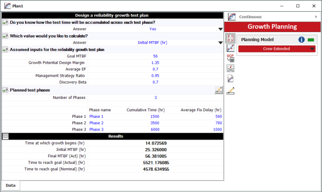
The input provided is the required MTBF goal of 56, the growth potential design margin of 1.35, the management strategy of 0.95 and the discovery beta of 0.7. The results show the initialization time,
, the initial MTBF, the final actual MTBF that can be reached for this growth program and the actual time when the MTBF goal is met. Note that in this case we provided the goal MTBF and solved for the initial MTBF.
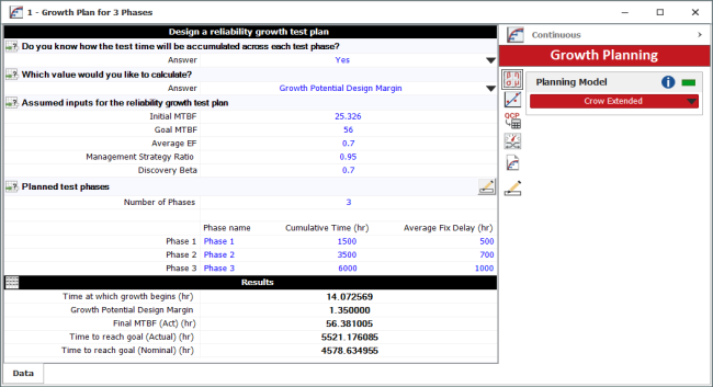
Different calculation options are available depending on the desired input and output. For example, we could provide the initial and goal MTBF to solve for the growth potential design margin, as shown in the figure below.
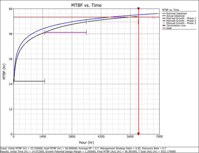
Click the Plot icon to generate a plot that shows the nominal and actual idealized growth curve, the test termination time, the MTBF goal and the planned growth for each phase, as shown in the figure below.
Growth Plan for 7 Phases
The reliability team of a product manufacturer is putting together a reliability growth plan for one of the new products under design. The team wants to create an overall reliability growth plan based on the Crow Extended model. The inputs to the model are the following:
- The requirement or goal MTBF is
hours.
- The growth potential design margin factor is
.
- The average effectiveness factor is
based on historical information for similar products developed by the company.
- The management strategy is
.
- The beta parameter for the discovery function,
of the type B failure modes is
, based on a data analysis of the previous product development project that was of similar nature.
- The test will be conducted in seven phases. The cumulative phase end times are
,
and
hours. The average fix delay for each phase is one week.
- For the first two phases, the plan is to test 1,000 hours per week, so the average fix delay in terms of test hours for phases 1 and 2 is
and
hours.
- For phases 3 and 4, the prototype test units are planned to be doubled, so the average fix delay in terms of test hours within one week is also going to be doubled, so we have:
and
hours.
- For phases 5 and 6, a second shift is going to be added, so the amount of test hours within a week is going to be doubled again. Therefore, the average fix delay in terms of test hours within one week is also going to be doubled:
and
hours. ***For the last phase, more units and weekend shifts are planned to be added, so the total test hours within one week are going to be 6,000 hours. In accordance, the average fix delay in terms of test hours will be
hours.
- For the first two phases, the plan is to test 1,000 hours per week, so the average fix delay in terms of test hours for phases 1 and 2 is
Determine the following: Construct a reliability growth plan using the Weibull++ software and make sure that the goal MTBF can be met within the total test hours allocated for growth testing. If not, make necessary changes in the phase durations in order to meet the goal.
Solution
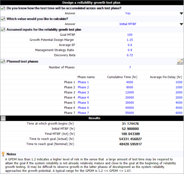
The following figure shows the planning inputs in Weibull++'s continuous growth planning folio.
The next figure shows the planning calculations based on the goal MTBF of 100 hours and the rest of the known inputs into the model. As seen by the planning calculation results, the final actual MTBF at the end of the seventh phase is 98.66 hours, which is less than the MTBF goal of 100 hours.
Also, the next figure shows that the nominal time to meet the MTBF goal is 48,420 hours, which is higher than the total test time that is currently planned to be allocated for reliability growth.
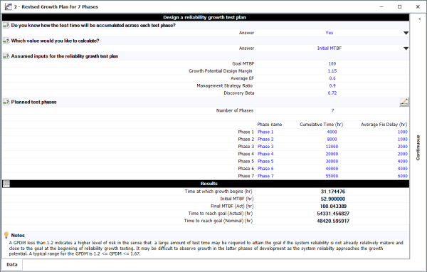
A new plan needs to be considered. The reliability team decides to increase the test time for phases 5 and 6 to be 10,000 hours each, instead of the 5,000 hours that were considered in the initial plan. Also, the team decides to increase the duration of the 7th phase to 15,000 hours. Since this is going to be achieved by testing for more calendar time in phases 5, 6 and 7, the average fix delay during those phases is the same as the one in the initial plan. The test time per week is not going to be affected, only more weeks will be added to the schedule. The next figure shows the revised plan, together with the calculated results. The actual time to meet the MTBF goal is now 54,331 hours. The final MTBF that can be achieved at the end of the 55,000 hours of growth testing is 100.04, which is slightly higher than the goal MTBF of 100 hours. The reliability team considers this plan as acceptable, since the MTBF goal will be met.
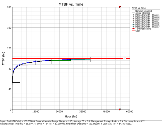
The next plot shows the overall reliability growth plan, with the nominal and actual growth curves, the MTBF goal line and the planned MTBF for each of the seven phases.
Growth Plan for 4 Phases
The reliability team of a product manufacturer has put together a reliability growth plan, based on the Crow Extended model, for one of their new products. The reliability growth model was constructed with the following inputs:
- The requirement or goal MTBF is
hours.
- The growth potential design margin factor is
.
- The average effectiveness factor is
- The management strategy is
.
- The beta parameter for the discovery function,
of the type B failure modes is
.
- The test is planned to be conducted in four phases. The cumulative phase end times are
,
and
. The average fix delay in terms of test hours for each phase is:
,
and
hours.
Determine the following:
- Plot the nominal and actual reliability growth curves for this program, using the Weibull++ software.
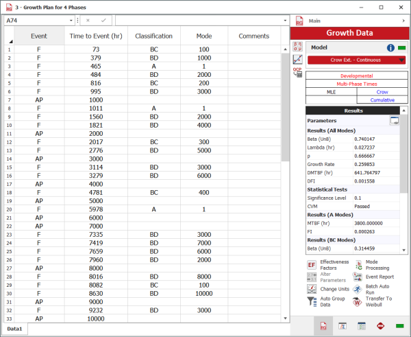
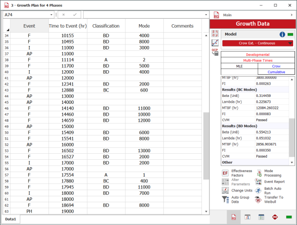
- The reliability program was initiated and actual test data from phase 1 is now available. The test data were analyzed using the Crow Extended - Continuous Evaluation model and the following figure shows the results.
Note that the I events, which represent the times for implementation of fixes for BD modes, occur at least 10,000 hours after the first occurrence of the specific BD mode. This is a reflection of the average fix delay being equal to 10,000 hours for the first test phase. Of course we could have some exceptions that could have been fixed before 10,000 hours after the first occurrence (i.e., discovery) of the mode, but on average, they should be fixed after 10,000 hours.
The same applies to the delayed fixes at the end of phase 1. On average there should be at least 10,000 test hours between the discovery of the failure mode and the implementation of a fix for that mode, so failure modes discovered after 9,000 hours of testing in the first phase cannot be implemented at the end of the first phase.
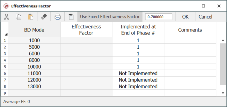
The figure below shows the effectiveness factor window. The record shows that the fixes for failure modes BD 11000, BD 12000 and BD 13000 are not implemented at the end of the first phase due to the fix delay. The effectiveness factor used is in accordance with the planning model and has been fixed to 0.7.
Construct a multi-phase graph that shows the analysis points for the test data in phase 1, as compared to the nominal and actual idealized growth curves for this reliability growth plan. Is the program on track, so far, as compared to the plan?
Solution
- The following figures show the plan inputs, phase durations and average fix delays as entered in Weibull++'s continuous growth planning folio, together with the results of the growth model.
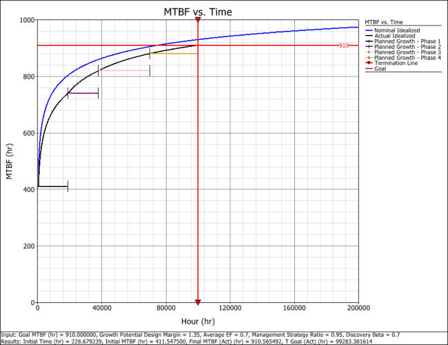
The next figure shows the nominal and actual idealized growth curves for this program, together with the program MTBF goal.
- The next step is to associate the reliability growth plan with the data from phase 1. To do that, right-click the
Multiplots heading in the current project explorer and choose
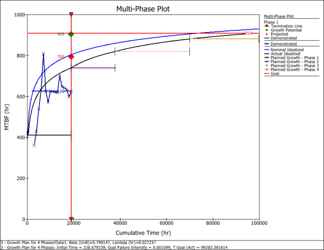
Add Multi-Phase Plot from the shortcut menu, then follow the wizard to specify the data sheet that contains the phase 1 data with the folio that defines the growth plan. The figure below shows the generated multi-phase plot, which brings together the reliability growth planning model with the actual test results. This plot shows the demonstrated MTBF for each analysis point during the first phase of testing. Analysis points for projected and growth potential MTBF can also be plotted. For this example, it can be said that the program is on track since the demonstrated MTBF of the first phase is higher than the planned MTBF for that phase.
The multi-phase plot can be updated continuously as the growth program progresses and more test data become available. In that manner, the reliability team can assess the actual reliability performance against the established goals.


![{\displaystyle {{t}_{0}}={{\left[{\frac {{{\lambda }_{I}}-{{\lambda }_{A}}-(1-d){{\lambda }_{B}}}{d\lambda \beta }}\right]}^{\tfrac {1}{\beta -1}}}\,\!}](https://en.wikipedia.org/api/rest_v1/media/math/render/svg/7fbb5e4f1fc2a74944b14c725fdc9e6276c54b50)

![{\displaystyle {{t}_{0}}={{\left[{\frac {{{\lambda }_{A}}+{{\lambda }_{B}}-{{\lambda }_{A}}-(1-d){{\lambda }_{B}}}{d\cdot \lambda \cdot \beta }}\right]}^{\tfrac {1}{\beta -1}}}\,\!}](https://en.wikipedia.org/api/rest_v1/media/math/render/svg/b68ea84e3238e3ffc917c72d2517a60f50eb6ce4)


![{\displaystyle {{t}_{N,G}}={{\left[{\frac {{{r}_{G}}-{{\lambda }_{A}}-(1-d){{\lambda }_{B}}}{d\cdot \lambda \cdot \beta }}\right]}^{\tfrac {1}{\beta -1}}}\,\!}](https://en.wikipedia.org/api/rest_v1/media/math/render/svg/7b995fd33b278184ab1ec551f30d68de10553e75)


![{\displaystyle {\begin{aligned}D(t)=\lambda {{t}^{(\beta -1)}}[1-\beta ]\end{aligned}}\,\!}](https://en.wikipedia.org/api/rest_v1/media/math/render/svg/66d930ad7b5477cd2a4aa140f5194fe3f1ca81d1)


![{\displaystyle {\begin{aligned}{{D}_{NI}}(t)=[{{C}_{NI}}(t)-{{r}_{NI}}(t)]=\lambda {{t}^{(\beta -1)}}[1-\beta ]\end{aligned}}\,\!}](https://en.wikipedia.org/api/rest_v1/media/math/render/svg/a36370b765f05ef6adfd85579f6ff93d442202d0)


![{\displaystyle {{r}_{AI}}(t)={{\lambda }_{A}}+(1-d){{\lambda }_{B}}+d\lambda \beta {{\left[\left({\frac {{{T}_{1}}-{{L}_{1}}}{{T}_{1}}}\right)t\right]}^{(\beta -1)}}{\text{ for }}0<t\leq {{T}_{1}}\,\!}](https://en.wikipedia.org/api/rest_v1/media/math/render/svg/b25c8a92fcc23f0050667ee329c968a936edb05d)


![{\displaystyle {{r}_{AI}}(T_{0}^{AIC})={{\lambda }_{A}}+(1-d){{\lambda }_{B}}+d\lambda \beta {{\left[\left({\frac {{{T}_{1}}-{{L}_{1}}}{{T}_{1}}}\right)T_{0}^{AIC}\right]}^{(\beta -1)}}\,\!}](https://en.wikipedia.org/api/rest_v1/media/math/render/svg/e875f6da86b73dba12cae5379fd0d4c8693ca046)

![{\displaystyle {{\lambda }_{A}}+(1-d){{\lambda }_{B}}+d\lambda \beta {{\left[\left({\frac {{{T}_{1}}-{{L}_{1}}}{{T}_{1}}}\right)T_{0}^{AIC}\right]}^{(\beta -1)}}={{\lambda }_{A}}+(1-d){{\lambda }_{B}}+d\lambda \beta t_{0}^{(\beta -1)}\,\!}](https://en.wikipedia.org/api/rest_v1/media/math/render/svg/8d5a0d2cbfc75bfa932270d8a74706f3181d32a4)


![{\displaystyle {{r}_{AI}}(t)={{\lambda }_{A}}+(1-d){{\lambda }_{B}}+d\lambda \beta {{\left[{{T}_{i-1}}-{{L}_{i-1}}+\left({\frac {{{T}_{i}}-{{L}_{i}}-{{T}_{i-1}}+{{L}_{i-1}}}{{{T}_{i}}-{{T}_{i-1}}}}\right)(t-{{T}_{i-1}})\right]}^{(\beta -1)}}\,\!}](https://en.wikipedia.org/api/rest_v1/media/math/render/svg/33782ccfa753731b611adef5121350f125b576ee)


![{\displaystyle {\begin{aligned}{{r}_{AI}}({{t}_{AC,G}})={{\lambda }_{A}}+(1-d){{\lambda }_{B}}+d\lambda \beta {{\left[{{T}_{i-1}}-{{L}_{i-1}}+\left({\frac {{{T}_{i}}-{{L}_{i}}-{{T}_{i-1}}+{{L}_{i-1}}}{{{T}_{i}}-{{T}_{i-1}}}}\right)({{t}_{AC,G}}-{{T}_{i-1}})\right]}^{(\beta -1)}}\end{aligned}}\,\!}](https://en.wikipedia.org/api/rest_v1/media/math/render/svg/d435db31b6593e3aecbda627c2b415db082c268a)


![{\displaystyle {\begin{aligned}{{r}_{G}}=&{{\lambda }_{A}}+(1-d){{\lambda }_{B}}\\&+d\lambda \beta {{\left[{{T}_{F-1}}-{{L}_{F-1}}+\left({\frac {{{T}_{F}}-{{L}_{F}}-{{T}_{F-1}}+{{L}_{F-1}}}{{{T}_{F}}-{{T}_{F-1}}}}\right)({{t}_{AC,G}}-{{T}_{F-1}})\right]}^{(\beta -1)}}\end{aligned}}\,\!}](https://en.wikipedia.org/api/rest_v1/media/math/render/svg/a02ab17e381cfd7c8de9a02379b79a6e231db7a3)

![{\displaystyle {{\left[{\frac {{{r}_{G}}-{{\lambda }_{A}}-(1-d){{\lambda }_{B}}}{d\lambda \beta }}\right]}^{\tfrac {1}{\beta -1}}}={{T}_{F-1}}-{{L}_{F-1}}+\left({\frac {{{T}_{F}}-{{L}_{i}}-{{T}_{F-1}}+{{L}_{F-1}}}{{{T}_{F}}-{{T}_{F-1}}}}\right)({{t}_{AC,G}}-{{T}_{F-1}})\,\!}](https://en.wikipedia.org/api/rest_v1/media/math/render/svg/6d9e13b72489a7c22f1a829c719e0a36200606c3)


![{\displaystyle {\begin{aligned}{{t}_{0}}=&{{\left[{\frac {{{\lambda }_{I}}-{{\lambda }_{A}}-(1-d){{\lambda }_{B}}}{d\lambda \beta }}\right]}^{\tfrac {1}{\beta -1}}}\\=&{{\left[{\frac {0.0394-0.001974-(1-0.7)0.0375}{0.7\cdot 0.1183\cdot 0.7}}\right]}^{\tfrac {1}{0.7-1}}}\end{aligned}}\,\!}](https://en.wikipedia.org/api/rest_v1/media/math/render/svg/0d60f1e51794c97ca12863fee6ccc684e5657365)


![{\displaystyle {{t}_{N,goal}}={{\left[{\frac {{{r}_{G}}-{{\lambda }_{A}}-(1-d){{\lambda }_{B}}}{d\lambda \beta }}\right]}^{\tfrac {1}{\beta -1}}}\,\!}](https://en.wikipedia.org/api/rest_v1/media/math/render/svg/892d7ae5dc979ce29b379ad25df5ea2589da5f5a)

![{\displaystyle {\begin{aligned}{{t}_{N,G}}=&{{\left[{\frac {0.01785-0.001974-(1-0.7)0.0375}{0.7\cdot 0.1184\cdot 0.7}}\right]}^{^{\tfrac {1}{\beta -1}}}}\\=&4578{\text{ hours}}\end{aligned}}\,\!}](https://en.wikipedia.org/api/rest_v1/media/math/render/svg/205f970206b38ae003b84b6da611ef118bd80e1f)


![{\displaystyle {\begin{aligned}{{r}_{AI,final}}(T)=&{{\lambda }_{A}}+(1-d){{\lambda }_{B}}\\&+d\lambda \beta {{\left[{{T}_{2}}-{{L}_{2}}+\left({\frac {{{T}_{3}}-{{L}_{3}}-{{T}_{2}}+{{L}_{2}}}{{{T}_{3}}-{{T}_{2}}}}\right)(T-{{T}_{2}})\right]}^{(\beta -1)}}\end{aligned}}\,\!}](https://en.wikipedia.org/api/rest_v1/media/math/render/svg/7c767f46dd4490fe5838ed1f6f3a59fd8d94798b)
![{\displaystyle {\begin{aligned}{{r}_{AI,final}}(T)=&0.0019+\left(1-0.7\right)0.0375+0.7\cdot 0.1184\cdot 0.7\\&\cdot {{\left[3500-700+\left({\frac {4500-1000-3500+700}{4500-3500}}\right)(4500-3500)\right]}^{(0.7-1)}}\end{aligned}}\,\!}](https://en.wikipedia.org/api/rest_v1/media/math/render/svg/e7b6521c353a0cb2873e7c166905f21d9cf49eaa)


![{\displaystyle {\begin{aligned}{{r}_{AI,final}}(T)=&0.0019+\left(1-0.7\right)0.0375+0.7\cdot 0.1184\cdot 0.7\\&\cdot {{\left[3500-700+\left({\frac {6000-1000-3500+700}{6000-3500}}\right)(6000-3500)\right]}^{(0.7-1)}}\end{aligned}}\,\!}](https://en.wikipedia.org/api/rest_v1/media/math/render/svg/cf3c56cc5d7c4f2b0c7a6f1e4f6f856437fd9416)


