Appendix B: Maximum Likelihood Estimation Example
MLE Statistical Background
If is a continuous random variable with
pdf:
where are
unknown constant parameters that need to be estimated, conduct an experiment and obtain
independent observations,
, which correspond in the case of life data analysis to failure times. The likelihood function (for complete data) is given by:
The logarithmic likelihood function is:
The maximum likelihood estimators (MLE) of
are obtained by maximizing
or
By maximizing
which is much easier to work with than
, the maximum likelihood estimators (MLE) of
are the simultaneous solutions of
equations such that:
Even though it is common practice to plot the MLE solutions using median ranks (points are plotted according to median ranks and the line according to the MLE solutions), this is not completely accurate. As it can be seen from the equations above, the MLE method is independent of any kind of ranks. For this reason, many times the MLE solution appears not to track the data on the probability plot. This is perfectly acceptable since the two methods are independent of each other, and in no way suggests that the solution is wrong.
Illustrating MLE Using the Exponential Distribution
- To estimate
for a sample of
units (all tested to failure), first obtain the likelihood function:
- Take the natural log of both sides:
- Obtain
, and set it equal to zero:
- Solve for
or:
Notes About
Note that the value of is an estimate because if we obtain another sample from the same population and re-estimate
, the new value would differ from the one previously calculated. In plain language,
is an estimate of the true value of ... How close is the value of our estimate to the true value? To answer this question, one must first determine the distribution of the parameter, in this case
. This methodology introduces a new term, confidence bound, which allows us to specify a range for our estimate with a certain confidence level. The treatment of confidence bounds is integral to reliability engineering, and to all of statistics. (Confidence bounds are covered in
Confidence Bounds.)
Illustrating MLE Using the Normal Distribution
To obtain the MLE estimates for the mean,
and standard deviation,
for the normal distribution, start with the
pdf of the normal distribution which is given by:
If are known times-to-failure (and with no suspensions), then the likelihood function is given by:
then:
Then taking the partial derivatives of
with respect to each one of the parameters and setting them equal to zero yields:
and:
Solving the above two derivative equations simultaneously yields:
and:
It should be noted that these solutions are valid only for data with no suspensions, (i.e., all units are tested to failure). In the case where suspensions are present or all units are not tested to failure, the methodology changes and the problem becomes much more complicated.
Illustrating with an Example of the Normal Distribution
If we had five units that failed at 10, 20, 30, 40 and 50 hours, the mean would be:
The standard deviation estimate then would be:
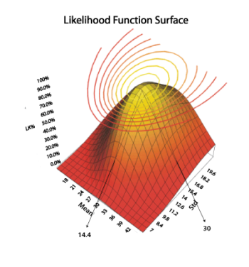
A look at the likelihood function surface plot in the figure below reveals that both of these values are the maximum values of the function.
This three-dimensional plot represents the likelihood function. As can be seen from the plot, the maximum likelihood estimates for the two parameters correspond with the peak or maximum of the likelihood function surface.


![{\displaystyle L({{T}_{1}},{{T}_{2}},...,{{T}_{N}}|{\bar {T}},{{\sigma }_{T}})=L={\underset {i=1}{\overset {N}{\mathop {\prod } }}}\,\left[{\frac {1}{{{\sigma }_{T}}{\sqrt {2\pi }}}}{{e}^{-{\tfrac {1}{2}}{{\left({\tfrac {{{T}_{i}}-{\bar {T}}}{{\sigma }_{T}}}\right)}^{2}}}}\right]\,\!}](https://en.wikipedia.org/api/rest_v1/media/math/render/svg/05bc19f100cc1dc2959fd87db361b54cec39d826)


