Randomization and Blocking in DOE
Randomization
The aspect of recording observations in an experiment in a random order is referred to as randomization. Specifically, randomization is the process of assigning the various levels of the investigated factors to the experimental units in a random fashion. An experiment is said to be completely randomized if the probability of an experimental unit to be subjected to any level of a factor is equal for all the experimental units. The importance of randomization can be illustrated using an example. Consider an experiment where the effect of the speed of a lathe machine on the surface finish of a product is being investigated. In order to save time, the experimenter records surface finish values by running the lathe machine continuously and recording observations in the order of increasing speeds. The analysis of the experiment data shows that an increase in lathe speeds causes a decrease in the quality of surface finish. However the results of the experiment are disputed by the lathe operator who claims that he has been able to obtain better surface finish quality in the products by operating the lathe machine at higher speeds. It is later found that the faulty results were caused because of overheating of the tool used in the machine. Since the lathe was run continuously in the order of increased speeds the observations were recorded in the order of increased tool temperatures. This problem could have been avoided if the experimenter had randomized the experiment and taken reading at the various lathe speeds in a random fashion. This would require the experimenter to stop and restart the machine at every observation, thereby keeping the temperature of the tool within a reasonable range. Randomization would have ensured that the effect of heating of the machine tool is not included in the experiment.
Blocking
Many times a factorial experiment requires so many runs that not all of them can be completed under homogeneous conditions. This may lead to inclusion of the effects of nuisance factors into the investigation. Nuisance factors are factors that have an effect on the response but are not of primary interest to the investigator. For example, two replicates of a two factor factorial experiment require eight runs. If four runs require the duration of one day to be completed, then the total experiment will require two days to be completed. The difference in the conditions on the two days may introduce effects on the response that are not the result of the two factors being investigated. Therefore, the day is a nuisance factor for this experiment. Nuisance factors can be accounted for using blocking. In blocking, experimental runs are separated based on levels of the nuisance factor. For the case of the two factor factorial experiment (where the day is a nuisance factor), separation can be made into two groups or blocks: runs that are carried out on the first day belong to block 1, and runs that are carried out on the second day belong to block 2. Thus, within each block conditions are the same with respect to the nuisance factor. As a result, each block investigates the effects of the factors of interest, while the difference in the blocks measures the effect of the nuisance factor. For the example of the two factor factorial experiment, a possible assignment of runs to the blocks could be as follows: one replicate of the experiment is assigned to block 1 and the second replicate is assigned to block 2 (now each block contains all possible treatment combinations). Within each block, runs are subjected to randomization (i.e., randomization is now restricted to the runs within a block). Such a design, where each block contains one complete replicate and the treatments within a block are subjected to randomization, is called randomized complete block design.
In summary, blocking should always be used to account for the effects of nuisance factors if it is not possible to hold the nuisance factor at a constant level through all of the experimental runs. Randomization should be used within each block to counter the effects of any unknown variability that may still be present.
Example
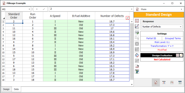
Consider the example discussed in General Full Factorial Design where the mileage of a sports utility vehicle was investigated for the effects of speed and fuel additive type. Now assume that the three replicates for this experiment were carried out on three different vehicles. To ensure that the variation from one vehicle to another does not have an effect on the analysis, each vehicle is considered as one block. See the experiment design in the following figure.

For the purpose of the analysis, the block is considered as a main effect except that it is assumed that interactions between the block and the other main effects do not exist. Therefore, there is one block main effect (having three levels - block 1, block 2 and block 3), two main effects (speed -having three levels; and fuel additive type - having two levels) and one interaction effect (speed-fuel additive interaction) for this experiment. Let
represent the block effects. The hypothesis test on the block main effect checks if there is a significant variation from one vehicle to the other. The statements for the hypothesis test are:
The test statistic for this test is:
where represents the mean square for the block main effect and
is the error mean square. The hypothesis statements and test statistics to test the significance of factors
(speed),
(fuel additive) and the interaction
(speed-fuel additive interaction) can be obtained as explained in the
example. The ANOVA model for this example can be written as:
where:
represents the overall mean effect
is the effect of the
th level of the block (
)
is the effect of the
th level of factor
(
)
is the effect of the
th level of factor
(
)
represents the interaction effect between
and
- and
represents the random error terms (which are assumed to be normally distributed with a mean of zero and variance of
)
In order to calculate the test statistics, it is convenient to express the ANOVA model of the equation given above in the form
. This can be done as explained next.
Expression of the ANOVA Model as y = ΧΒ + ε
Since the effects ,
,
, and
are defined as deviations from the overall mean, the following constraints exist.
Constraints on are:
Therefore, only two of the effects are independent. Assuming that
and
are independent,
. (The null hypothesis to test the significance of the blocks can be rewritten using only the independent effects as
.) In DOE folios, the independent block effects,
and
, are displayed as Block[1] and Block[2], respectively.
Constraints on are:
Therefore, only two of the effects are independent. Assuming that
and
are independent,
. The independent effects,
and
, are displayed as A[1] and A[2], respectively.
Constraints on
are:
Therefore, only one of the effects is independent. Assuming that
is independent,
. The independent effect,
, is displayed as B:B.
Constraints on
are:
The last five equations given above represent four constraints as only four of the five equations are independent. Therefore, only two out of the six
effects are independent. Assuming that
and
are independent, we can express the other four effects in terms of these effects. The independent effects,
and
, are displayed as A[1]B and A[2]B, respectively.
The regression version of the ANOVA model can be obtained using indicator variables. Since the block has three levels, two indicator variables,
and
, are required, which need to be coded as shown next:
Factor has three levels and two indicator variables,
and
, are required:
Factor has two levels and can be represented using one indicator variable,
, as follows:
The interaction will be represented by
and
. The regression version of the ANOVA model can finally be obtained as:
In matrix notation this model can be expressed as:
- or:
Knowing ,
and
, the sum of squares for the ANOVA model and the extra sum of squares for each of the factors can be calculated. These are used to calculate the mean squares that are used to obtain the test statistics.
Calculation of the Sum of Squares for the Model
The model sum of squares, , for the ANOVA model of this example can be obtained as:
Since seven effect terms (,
,
,
,
,
and
) are used in the model the number of degrees of freedom associated with
is seven (
).
The total sum of squares can be calculated as:
Since there are 18 observed response values, the number of degrees of freedom associated with the total sum of squares is 17 (). The error sum of squares can now be obtained:
The number of degrees of freedom associated with the error sum of squares is:
Since there are no true replicates of the treatments (as can be seen from the design of the previous figure, where all of the treatments are seen to be run just once), all of the error sum of squares is the sum of squares due to lack of fit. The lack of fit arises because the model used is not a full model since it is assumed that there are no interactions between blocks and other effects.
Calculation of the Extra Sum of Squares for the Factors
The sequential sum of squares for the blocks can be calculated as:
where is the matrix of ones,
is the hat matrix, which is calculated using
, and
is the matrix containing only the first three columns of the
matrix. Thus
Since there are two independent block effects, and
, the number of degrees of freedom associated with
is two (
).
Similarly, the sequential sum of squares for factor
can be calculated as:
Sequential sum of squares for the other effects are obtained as
and
.
Calculation of the Test Statistics
Knowing the sum of squares, the test statistics for each of the factors can be calculated. For example, the test statistic for the main effect of the blocks is:
The value corresponding to this statistic based on the
distribution with 2 degrees of freedom in the numerator and 10 degrees of freedom in the denominator is:
Assuming that the desired significance level is 0.1, since
value > 0.1, we fail to reject
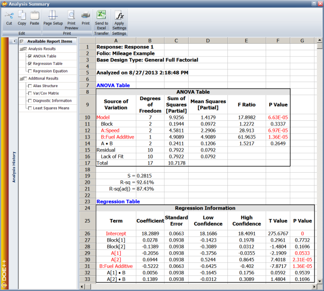
and conclude that there is no significant variation in the mileage from one vehicle to the other. Statistics to test the significance of other factors can be calculated in a similar manner. The complete analysis results obtained from the DOE folio for this experiment are presented in the following figure.


![{\displaystyle \left[{\begin{matrix}17.3\\18.9\\17.1\\18.7\\19.1\\18.8\\17.8\\18.2\\.\\.\\18.3\\\end{matrix}}\right]=\left[{\begin{matrix}1&1&0&1&0&1&1&0\\1&1&0&0&1&1&0&1\\1&1&0&-1&-1&1&-1&-1\\1&1&0&1&0&-1&-1&0\\1&1&0&0&1&-1&0&-1\\1&1&0&-1&-1&-1&1&1\\1&0&1&1&0&1&1&0\\1&0&1&0&1&1&0&1\\.&.&.&.&.&.&.&.\\.&.&.&.&.&.&.&.\\1&-1&-1&-1&-1&-1&1&1\\\end{matrix}}\right]\left[{\begin{matrix}\mu \\{{\zeta }_{1}}\\{{\zeta }_{2}}\\{{\tau }_{1}}\\{{\tau }_{2}}\\{{\delta }_{1}}\\{{(\tau \delta )}_{11}}\\{{(\tau \delta )}_{21}}\\\end{matrix}}\right]+\left[{\begin{matrix}{{\epsilon }_{111}}\\{{\epsilon }_{121}}\\{{\epsilon }_{131}}\\{{\epsilon }_{112}}\\{{\epsilon }_{122}}\\{{\epsilon }_{132}}\\{{\epsilon }_{211}}\\{{\epsilon }_{221}}\\.\\.\\{{\epsilon }_{332}}\\\end{matrix}}\right]\,\!}](https://en.wikipedia.org/api/rest_v1/media/math/render/svg/7aa45cbe8c23fde3bbc989d4923324fa7e47a4c9)


![{\displaystyle {\begin{aligned}&S{{S}_{TR}}=&{{y}^{\prime }}[H-({\frac {1}{{{n}_{a}}\cdot {{n}_{b}}\cdot m}})J]y\\&=&{{y}^{\prime }}[H-({\frac {1}{18}})J]y\\&=&9.9256\end{aligned}}\,\!}](https://en.wikipedia.org/api/rest_v1/media/math/render/svg/8e1eda1fa5b91c390d2e82d83dbdfa5de4183a11)

![{\displaystyle {\begin{aligned}&S{{S}_{T}}=&{{y}^{\prime }}[I-({\frac {1}{{{n}_{a}}\cdot {{n}_{b}}\cdot m}})J]y\\&=&{{y}^{\prime }}[H-({\frac {1}{18}})J]y\\&=&10.7178\end{aligned}}\,\!}](https://en.wikipedia.org/api/rest_v1/media/math/render/svg/1d3188ffc1a06d7803c39efcde2f6f4a7a4927aa)


![{\displaystyle {\begin{aligned}S{{S}_{Block}}=&S{{S}_{TR}}(\mu ,{{\zeta }_{1}},{{\zeta }_{2}})-S{{S}_{TR}}(\mu )\\=&{{y}^{\prime }}[{{H}_{\mu ,{{\zeta }_{1}},{{\zeta }_{2}}}}-({\frac {1}{18}})J]y-0\end{aligned}}\,\!}](https://en.wikipedia.org/api/rest_v1/media/math/render/svg/c9ed7d10be19b97e153c50ac238161241405cdf7)


![{\displaystyle {\begin{aligned}S{{S}_{Block}}=&{{y}^{\prime }}[{{H}_{\mu ,{{\zeta }_{1}},{{\zeta }_{2}}}}-({\frac {1}{18}})J]y-0\\=&0.1944-0\\=&0.1944\end{aligned}}\,\!}](https://en.wikipedia.org/api/rest_v1/media/math/render/svg/c39c98c98a0a42df6505f1476af728164075a07a)


![{\displaystyle {\begin{aligned}S{{S}_{A}}=&S{{S}_{TR}}(\mu ,{{\zeta }_{1}},{{\zeta }_{2}},{{\tau }_{1}},{{\tau }_{2}})-S{{S}_{TR}}(\mu ,{{\zeta }_{1}},{{\zeta }_{2}})\\=&{{y}^{\prime }}[{{H}_{\mu ,{{\zeta }_{1}},{{\zeta }_{2}},{{\tau }_{1}},{{\tau }_{2}}}}-({\frac {1}{18}})J]y-{{y}^{\prime }}[{{H}_{\mu ,{{\zeta }_{1}},{{\zeta }_{2}}}}-({\frac {1}{18}})J]y\\=&4.7756-0.1944\\=&4.5812\end{aligned}}\,\!}](https://en.wikipedia.org/api/rest_v1/media/math/render/svg/3d34db2cf72f9a5639e8e7df6ff61344fa16b92f)


