Design Evaluation and Power Study
In general, there are three stages in applying design of experiments (DOE) to solve an issue: designing the experiment, conducting the experiment, and analyzing the data. The first stage is very critical. If the designed experiment is not efficient, you are unlikely to obtain good results. It is very common to evaluate an experiment before conducting the tests. A design evaluation often focuses on the following four properties:
- The alias structure. Are main effects and two-way interactions in the experiment aliased with each other? What is the resolution of the design?
- The orthogonality. An orthogonal design is always preferred. If a design is non-orthogonal, how are the estimated coefficients correlated?
- The optimality. A design is called "optimal" if it can meet one or more of the following criteria:
- D-optimality: minimize the determinant of the variance-covariance matrix.
- A-optimality: minimize the trace of the variance-covariance matrix.
- V-optimality: minimize the average prediction variance in the design space.
- The power (or its inverse, Type II error). Power is the probability of detecting an effect through experiments when it is indeed active. A design with low power for main effects is not a good design.
In the following sections, we will discuss how to evaluate a design according to these four properties.
Alias Structure
To reduce the sample size in an experiment, we usually focus only on the main effects and lower-order interactions, while assuming that higher-order interactions are not active. For example, screening experiments are often conducted with a number of runs that barely fits the main effect-only model. However, due to the limited number of runs, the estimated main effects often are actually combined effects of main effects and interaction effects. In other words the estimated main effects are aliased with interaction effects. Since these effects are aliased, the estimated main effects are said to be biased. If the interaction effects are large, then the bias will be significant. Thus, it is very important to find out how all the effects in an experiment are aliased with each other. A design's alias structure is used for this purpose, and its calculation is given below.
Assume the matrix representation of the true model for an experiment is:
If the model used in a screening experiment is a reduced one, as given by:
then, from this experiment, the estimated
is biased. This is because the ordinary least square estimator of
is:
As discussed in [Wu, 2000], the expected value of this estimator is:
where is called the
alias matrix of the design. For example, for a three factorial screening experiment with four runs, the design matrix is:
-
A B C -1 -1 1 1 -1 -1 -1 1 -1 1 1 1
If we assume the true model is:
and the used model (i.e., the model used in the experiment data analysis) is:
then and
. The alias matrix
A is calculated as:
-
AB AC BC ABC I 0 0 0 1 A 0 0 1 0 B 0 1 0 0 C 1 0 0 0
Sometimes, we also put in the above matrix. Then the
A matrix becomes:
-
I A B C AB AC BC ABC I 1 0 0 0 0 0 0 1 A 0 1 0 0 0 0 1 0 B 0 0 1 0 0 1 0 0 C 0 0 0 1 1 0 0 0
For the terms included in the used model, the alias structure is:
From the alias structure and the definition of resolution, we know this is a resolution III design. The estimated main effects are aliased with two-way interactions. For example, A is aliased with BC. If, based on engineering knowledge, the experimenter suspects that some of the interactions are important, then this design is unacceptable since it cannot distinguish the main effect from important interaction effects.
For a designed experiment it is better to check its alias structure before conducting the experiment to determine whether or not some of the important effects can be clearly estimated.
Orthogonality
Orthogonality is a model-related property. For example, for a main effect-only model, if all the coefficients estimated through ordinary least squares estimation are not correlated, then this experiment is an orthogonal design for main effects. An orthogonal design has the minimal variance for the estimated model coefficients. Determining whether a design is orthogonal is very simple. Consider the following model:
The variance and covariance matrix for the model coefficients is:
where is the variance of the error. When all the factors in the model are quantitative factors or all the factors are 2 levels,
is a regular symmetric matrix . The diagonal elements of it are the variances of model coefficients, and the off-diagonal elements are the covariance among these coefficients. When some of the factors are qualitative factors with more than 2 levels,
is a block symmetric matrix. The block elements in the diagonal represent the variance and covariance matrix of the qualitative factors, and the off-diagonal elements are the covariance among all the coefficients.
Therefore, to check if a design is orthogonal for a given model, we only need to check matrix :. For the example used in the previous section, if we assume the main effect-only model is used, then
is:
-
I A B C I 0.25 0 0 0 A 0 0.25 0 0 B 0 0 0.25 0 C 0 0 0 0.25
Since all the off-diagonal elements are 0, the design is an orthogonal design for main effects. For an orthogonal design, it is also true that the diagonal elements are 1/n, where n is the number of total runs.
When there are qualitative factors with more than 2 levels in the model,
will be a block symmetric matrix. For example, assume we have the following design matrix.
-
Run Order A B 1 -1 1 2 -1 1 3 -1 1 4 -1 2 5 -1 2 6 -1 2 7 -1 3 8 -1 3 9 -1 3 10 1 1 11 1 1 12 1 1 13 1 2 14 1 2 15 1 2 16 1 3 17 1 3 18 1 3
Factor B has 3 levels, so 2 indicator variables are used in the regression model. The
matrix for a model with main effects and the interaction is:
-
I A B[1] B[2] AB[1] AB[2] I 0.0556 0 0 0 0 0 A 0 0.0556 0 0 0 0 B[1] 0 0 0.1111 -0.0556 0 0 B[2] 0 0 -0.0556 0.1111 0 0 AB[1] 0 0 0 0 0.1111 -0.0556 AB[2] 0 0 0 0 -0.0556 0.1111
The above matrix shows this design is orthogonal since it is a block diagonal matrix.
For an orthogonal design for a given model, all the coefficients in the model can be estimated independently. Dropping one or more terms from the model will not affect the estimation of other coefficients and their variances. If a design is not orthogonal, it means some of the terms in the model are correlated. If the correlation is strong, then the statistical test results for these terms may not be accurate.
VIF (variance inflation factor) is used to examine the correlation of one term with other terms. The VIF is commonly used to diagnose multicollinearity in regression analysis. As a rule of thumb, a VIF of greater than 10 indicates a strong correlation between some of the terms. VIF can be simply calculated by:
For more detailed discussion on VIF, please see Multiple Linear Regression Analysis.
Optimality
Orthogonal design is always ideal. However, due to the constraints on sample size and cost, it is sometimes not possible. If this is the case, we want to get a design that is as orthogonal as possible. The so-called D-efficiency is used to measure the orthogonality of a two level factorial design. It is defined as:
- D-efficiency
where p is the number of coefficients in the model and n is the total sample size. D represents the determinant.
is the
information matrix of a design. When you compare two different screening designs, the one with a larger determinant of
is usually better.
D-efficiency can be used for comparing two designs. Other alphabetic optimal criteria are also used in design evaluation. If a model and the number of runs are given, an optimal design can be found using computer algorithms for one of the following optimality criteria:
- D-optimality: maximize the determinant of the information matrix
. This is the same as minimizing the determinant of the variance-covariance matrix
.
- A-optimality: minimize the trace of the variance-covariance matrix
. The trace of a matrix is the sum of all its diagonal elements.
- V-optimality (or I-optimality): minimize the average prediction variance within the design space.
The determinant of and the trace of
are given in the design evaluation in the DOE folio. V-optimality is not yet included.
Power Study
Power calculation is another very important topic in design evaluation. When designs are balanced, calculating the power (which, you will recall, is the probability of detecting an effect when that effect is active) is straightforward. However, for unbalanced designs, the calculation can be very complicated. We will discuss methods for calculating the power for a given effect for both balanced and unbalanced designs.
Power Study for Single Factor Designs (One-Way ANOVA)
Power is related to Type II error in hypothesis testing and is commonly used in statistical process control (SPC). Assume that at the normal condition, the output of a process follows a normal distribution with a mean of 10 and a standard deviation of 1.2. If the 3-sigma control limits are used and the sample size is 5, the control limits (assuming a normal distribution) for the X-bar chart are:
If a calculated mean value from a sampling group is outside of the control limits, then the process is said to be out of control. However, since the mean value is from a random process following a normal distribution with a mean of 10 and standard derivation of
, even when the process is under control, the sample mean still can be out of the control limits and cause a false alarm. The probability of causing a false alarm is called
Type I error (or significance level or risk level). For this example, it is:
Similarly, if the process mean has shifted to a new value that means the process is indeed out of control (e.g., 12), applying the above control chart, the sample mean can still be within the control limits, resulting in a failure to detect the shift. The probability of causing a misdetection is called Type II error. For this example, it is:
Power is defined as 1-Type II error. In this case, it is 0.766302. From this example, we can see that Type I and Type II errors are affected by sample size. Increasing sample size can reduce both errors. Engineers usually determine the sample size of a test based on the power requirement for a given effect. This is called the Power and Sample Size issue in design of experiments.
Power Calculation for Comparing Two Means
For one factor design, or one-way ANOVA, the simplest case is to design an experiment to compare the mean values at two different levels of a factor. Like the above control chart example, the calculated mean value at each level (in control and out of control) is a random variable. If the two means are different, we want to have a good chance to detect it. The difference of the two means is called the effect of this factor. For example, to compare the strength of a similar rope from two different manufacturers, 5 samples from each manufacturer are taken and tested. The test results (in newtons) are given below.
-
M1 M2 123 99 134 103 132 100 100 105 98 97
For this data, the ANOVA results are:
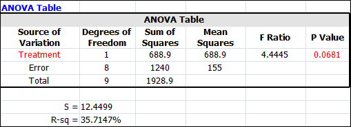
The standard deviation of the error is 12.4499 as shown in the above screenshot. and the t-test results are:
-
Mean Comparisons Contrast Mean Difference Pooled Standard Error Low CI High CI T Value P Value M1 - M2 16.6 7.874 -1.5575 34.7575 2.1082 0.0681
Since the p value is 0.0681, there is no significant difference between these two vendors at a significance level of 0.05 (since .0681 > 0.05). However, since the samples are randomly taken from the two populations, if the true difference between the two vendors is 30, what is the power of detecting this amount of difference from this test?
To answer this question: first, from the significance level of 0.05, let's calculate the critical limits for the t-test. They are:
Define the mean of each vendor as
and
. Then the difference between the estimated sample means is:
Under the null hypothesis (the two vendors are the same), the t statistic is:
Under the alternative hypothesis when the true difference is 30, the calculated
t statistic is from a non-central t distribution with non-centrality parameter
of:
The Type II error is
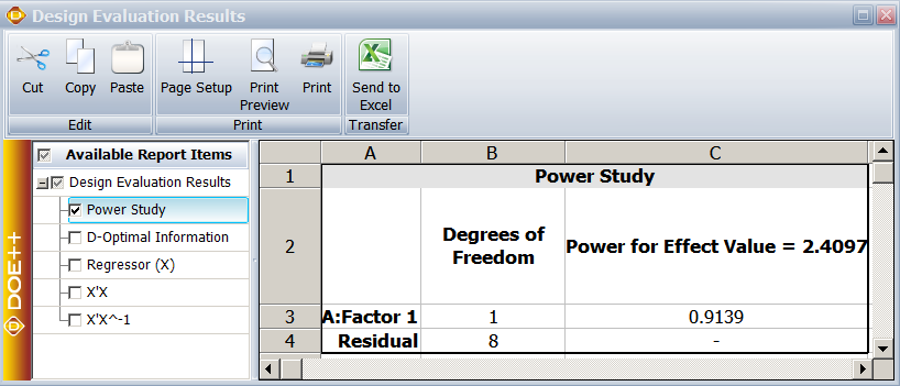
. So the power is 1-0.08609 =0.91391.
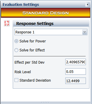
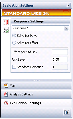
In a DOE folio, the Effect for the power calculation is entered as the multiple of the standard deviation of error. So effect of 30 is
standard deviation. This information is illustrated below.
and the calculated power for this effect is:
As we know, the square of a t distribution is an F distribution. The above ANOVA table uses the F distribution and the above "mean comparison" table uses the t distribution to calculate the p value. The ANOVA table is especially useful when conducting multiple level comparisons. We will illustrate how to use the F distribution to calculate the power for this example.
At a significance level of 0.05, the critical value for the F distribution is:
Under the alternative hypothesis when the true difference of these 2 vendors is 30, the calculated
f statistic is from a non-central F distribution with non-centrality parameter
.
The Type II error is
. So the power is 1-0.08609 = 0.91391. This is the same as the value we calculated using the non-central t distribution.
Power Calculation for Comparing Multiple Means: Balanced Designs
When a factor has only two levels, as in the above example, there is only one effect of this factor, which is the difference of the means at these two levels. However, when there are multiple levels, there are multiple paired comparisons. For example, if there are
r levels for a factor, there are
paired comparisons. In this case, what is the power of detecting a given difference among these comparisons?
In a DOE folio, the power for a multiple level factor is defined as follows: given the largest difference among all the level means is, power is the smallest probability of detecting this difference at a given significance level.
For example, if a factor has 4 levels and
is 3, there are many scenarios that the largest difference among all the level means will be 3. The following table gives 4 possible scenarios.
-
Case M1 Μ2 M3 M4 1 24 27 25 26 2 25 25 26 23 3 25 25 25 28 4 25 25 26.5 23.5
For all 4 cases, the largest difference among the means is the same: 3. The probability of detecting
(individual power) can be calculated using the method in the previous section for each case. It has been proven in
[Kutner etc 2005, Guo etc 2012] that when the experiment is balanced, case 4 gives the lowest probability of detecting a given amount of effect. Therefore, the individual power calculated for case 4 is also the power for this experiment. In case 4, all but two factor level means are at the grand mean, and the two remaining factor level means are equally spaced around the grand mean. Is this a general pattern? Can the conclusion from this example be applied to general cases of balanced design?
To answer these questions, let's illustrate the power calculation mathematically. In one factor design or one-way ANOVA, a level is also traditionally called a treatment. The following linear regression model is used to model the data:
where
is the
th observation at the
th treatment and
First, let's define the problem of power calculation.
The power calculation of an experiment can be mathematically defined as:
where is the number of levels,
is the total samples, α is the significance level of the hypothesis testing, and
is the critical value. The obtained minimal of the objective function in the above optimization problem is the power. The above optimization is the same as minimizing
, the non-centrality parameter, since all the other variables in the non-central F distribution are fixed.
Second, let's relate the level means with the regression coefficients.
Using the regression model, the mean response at the ith factor level is:
The difference of level means can also be defined using the
values. For example, let
, then:
Using
, the non-centrality parameter
can be calculated as:
where
and
is the variance and covariance matrix for
. When the design is balanced, we know:
where n is the sample size at each level.
Third, let's solve the optimization problem for balanced designs.
The power is calculated when
is at its minimum. Therefore, for balanced designs, the optimization issue becomes:
The two equations in the constraint represent two cases. Without losing generality,
is set to 1 in the following discussion.
Case 1:
, that is, the last level of the factor does not appear in the difference of level means.
For example, let
.
. The optimal solution is
,
,
for
. This result means that at the optimal solution,
,
,
,
.
Case 2: In this case, one level in the comparisons is the last level of the factor in the largest difference of
.
For example, let .
The optimal solution is
,
for
. This result means that at the optimal solution,
,
, and
,
.
The proof for Case 1 and Case 2 is given in [Guo IEEM2012]. The results for Case 1 and Case 2 show that when one of the level means (adjusted by the grand mean) is
, another level mean is -
and the rest level means are 0, the calculated power is the smallest power among all the possible scenarios. This result is the same as the observation for the 4-case example given at the beginning at this section.
Let's use the above optimization method to solve the example given in the previous section. In that example, the factor has 2 levels; the sample size is 5 at each level; the estimated
; and
. The regression model is:
Since the sample size is 5,
. From the above discussion, we know that when
, we get the minimal non-centrality parameter
. This value is the same as what we got in the previous section using the non-central t and F distributions. Therefore, the method discussed in this section is a general method and can be used for cases with 2 level and multiple level factors. The previous non-central t and F distribution method is only for cases with 2 level factors.
A 4 level balanced design example
Assume an engineer wants to compare the performance of 4 different materials. Each material is a level of the factor. The sample size for each level is 15 and the standard deviation
is 10. The engineer wants to calculate the power of this experiment when the largest difference among the materials is 15. If the power is less than 80%, he also wants to know what the sample size should be in order to obtain a power of 80%. Assume the significant level is 5%.
Step 1: Build the linear regression model. Since there are 4 levels, we need 3 indicator variables. The model is:
Step 2: Since the sample size is 15 and
is 10:
Step 3: Since there are 4 levels, there are 6 paired comparisons. For each comparison, the optimal
is:
-
ID Paired Comparison beta1 beta2 beta3 1 Level 1- Level 2 0.5 -0.5 0 2 Level 1- Level 3 0.5 0 -0.5 3 Level 1- Level 4 0.5 0 0 4 Level 2- Level 3 0 0.5 -0.5 5 Level 2- Level 4 0 0.5 0 6 Level 3- Level 4 0 0 0.5
Step 4: Calculate the non-centrality parameter for each of the 6 solutions:
The diagonal elements are the non-centrality parameter from each paired comparison. Denoting them as
, the power should be calculated using
. Since the design is balanced, we see here that all the
are the same.
Step 5: Calculate the critical F value.
Step 6: Calculate the power for this design using the non-central F distribution.
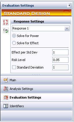
Since the power is greater than 80%, the sample size of 15 is sufficient. Otherwise, the sample size should be increased in order to achieve the desired power requirement. The settings and results in the DOE folio are given below.
Power Calculation for Comparing Multiple Means: Unbalanced Designs
If the design is not balanced, the non-centrality parameter does not have the simple expression of
, since
will not have the simpler format seen in balanced designs. The optimization thus becomes more complicated. For each paired comparison, we need to solve an optimization problem by assuming this comparison has the largest difference. For example, assuming the ith comparison
has the largest difference, we need to solve the following problem:
In total, we need to solve optimization problems and use the smallest
among all the solutions to calculate the power of the experiment. Clearly, the calculation will be very expensive.
In a DOE folio, instead of calculating the exact solution, we use the optimal
for a balanced design to calculate the approximated power for an unbalanced design. It can be seen that the optimal
for a balanced design also can satisfy all the constraints for an unbalanced design. Therefore, the approximated power is always higher than the unknown true power when the design is unbalanced.
A 3-level unbalanced design example: exact solution
Assume an engineer wants to compare the performance of three different materials. 4 samples are available for material A, 5 samples for material B and 13 samples for material C. The responses of different materials follow a normal distribution with a standard deviation of
. The engineer is required to calculate the power of detecting difference of 1
among all the level means at a significance level of 0.05.
From the design matrix of the test,
and
are calculated as:
,
There are 3 paired comparisons. They are
,
and
.
If the first comparison
has the largest level mean difference of 1
, then the optimization problem becomes:
The optimal solution is , and the optimal
.
If the second comparison
has the largest level mean difference, then the optimization is similar to the above problem. The optimal solution is
;
and the optimal
.
If the third comparison
has the largest level mean difference, then the optimal solution is
; {{\beta }_{2}}=0.57407\,\!</math> and the optimal
.
From the definition of power, we know that the power of a design should be calculated using the smallest non-centrality parameter of all possible outcomes. In this example, it is
. Since the significance level is 0.05, the critical value for the F test is
. The power for this example is:
A 3-level unbalanced design example: approximated solution
For the above example, we can get the approximated power by using the optimal
of a balanced design. If the design is balanced, the optimal solution will be:
-
Solution ID Paired Comparison β1 β2 1 u1-u2 0.5 -0.5 2 u1-u3 0.5 0 3 u2-u3 0 0.5
Therefore:
Since the design is unbalanced, use
from the above example to get:
The smallest
is 2.238636. For this example, it is very close to the exact solution 2.22222 given in the previous calculation. The approximated power is:
This result is a little larger than the exact solution of 0.2162.
In practical cases, the above method can be applied to quickly check the power of a design. If the calculated power cannot meet the required value, the true power definitely will not meet the requirement, since the calculated power using this procedure is always equal to (for balanced designs) or larger than (for unbalanced designs) the true value.
The result in the DOE folio for this example is given as:
-
Power Study Degrees of Freedom Power for Max Difference = 1 A:Factor 1 2 0.2174 Residual 19 -
Power Study for 2 Level Factorial Designs
For 2 level factorial designs, each factor (effect) has only one coefficient. The linear regression model is:
The model can include main effect terms and interaction effect terms. Each
can be -1 (the low level) or +1 (the high level). The effect of a main effect term is defined as the difference of the mean value of Y at
and
. Please notice that all the factor values here are coded values. For example, the effect of
is defined by:
Similarly, the effect of an interaction term is also defined as the difference of the mean values of Y at the interaction terms of +1 and -1. For example, the effect of
is:
Therefore, if the effect of a term that we want to calculate the power for is
, then the corresponding coefficient
must be
. Therefore, the non-centrality parameter for each term in the model for a 2 level factorial design can be calculated as
Once
is calculated, we can use it to calculate the power. If the design is balanced, the power of terms with the same order will be the same. In other words, all the main effects have the same power and all the k-way (k=2, 3, 4, ...) interactions have the same power.
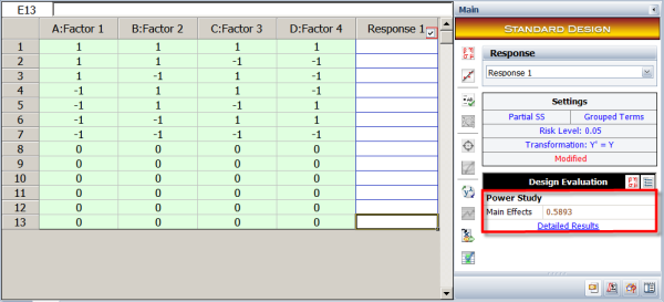
Example: Due to the constraints of sample size and cost, an engineer can run only the following 13 tests for a 4 factorial design:
-
Run A B C D 1 1 1 1 1 2 1 1 -1 -1 3 1 -1 1 -1 4 -1 1 1 -1 5 -1 1 -1 1 6 -1 -1 1 1 7 -1 -1 -1 -1 8 0 0 0 0 9 0 0 0 0 10 0 0 0 0 11 0 0 0 0 12 0 0 0 0 13 0 0 0 0
Before doing the tests, he wants to evaluate the power for each main effect. Assume the amount of effect he wants to perform a power calculation for is 2
. The significance level is 0.05.
Step 1: Calculate the variance and covariance matrix for the model coefficients. The main effect-only model is:
For this model:
The value for is
-
-
-
-
beta0 beta1 beta2 beta3 beta4 beta0 0.083333 0.020833 -0.02083 -0.02083 0.020833 beta1 0.020833 0.161458 -0.03646 -0.03646 0.036458 beta2 -0.02083 -0.03646 0.161458 0.036458 -0.03646 beta3 -0.02083 -0.03646 0.036458 0.161458 -0.03646 beta4 0.020833 0.036458 -0.03646 -0.03646 0.161458
-
-
-
The diagonal elements are the variances for the coefficients.
Step 2: Calculate the non-centrality parameter for each term. In this example, all the main effect terms have the same variance, so they have the same non-centrality parameter value.
Step 3: Calculate the critical value for the F test. It is:
Step 4: Calculate the power for each main effect term. For this example, the power is the same for all of them:
The settings and results in the DOE folio are given below.
In general, the calculated power for each term will be different for unbalanced designs. However, the above procedure can be applied for both balanced and unbalanced 2 level factorial designs.
Power Study for General Level Factorial Designs
For a quantitative factor X with more than 2 levels, its effect is defined as:
This is the difference of the expected Y values at its defined high and low level. Therefore, a quantitative factor can always be treated as a 2 level factor mathematically, regardless of its defined number of levels. A quantitative factor has only 1 term in the regression equation.
For a qualitative factor with more than 2 levels, it has more than 1 term in the regression equation. Like in the multiple level 1 factor designs, a qualitative factor with r levels will have r-1 terms in the linear regression equation. Assume there are 2 factors in a design. Factor A has 3 levels and factor B has 3 levels, the regression equation for this design is:
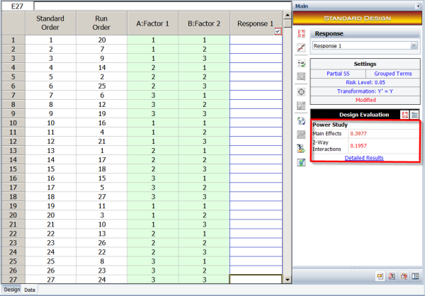
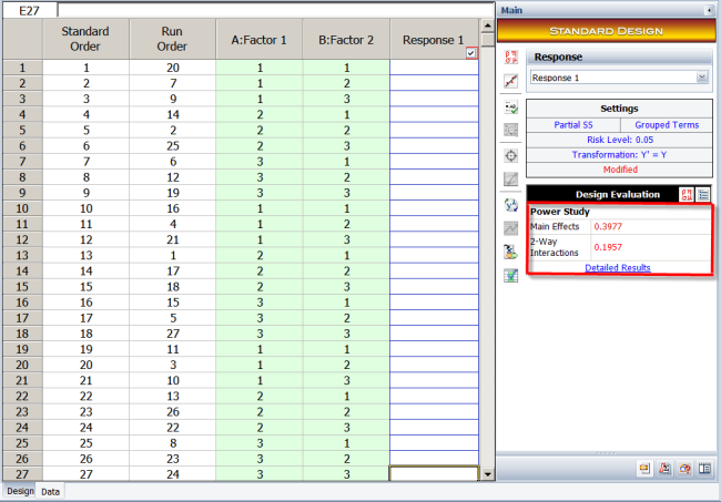
There are 2 regression terms for each main effect, and 4 regression terms for the interaction effect. We will use the above equation to explain how the power for the main effects and interaction effects is calculated in the DOE folio. The following balanced design is used for the calculation:
-
Run A B Run A B 1 1 1 14 2 2 2 1 2 15 2 3 3 1 3 16 3 1 4 2 1 17 3 2 5 2 2 18 3 3 6 2 3 19 1 1 7 3 1 20 1 2 8 3 2 21 1 3 9 3 3 22 2 1 10 1 1 23 2 2 11 1 2 24 2 3 12 1 3 25 3 1 13 2 1 26 3 2 27 3 3
Power Study for Main Effects
Let's use factor A to show how the power is defined and calculated for the main effects. For the above design, if we ignore factor B, then it becomes a 1 factor design with 9 samples at each level. Therefore, the same linear regression model and power calculation method as discussed for 1 factor designs can be used to calculate the power for the main effects for this multiple level factorial design.
Since A has 3 levels, it has 3 paired comparisons:
;
and
.
is the average of the responses at the ith level. However, these three contrasts are not independent, since
. We are interested in the largest difference among all the contrasts. Let
. Power is defined as the probability of detecting a given
in an experiment. Using the linear regression equation, we get:
Just as for the 1 factor design, we know the optimal solutions are:
when
is the largest difference
;
when
is the largest difference
and
when
is the largest difference
. For each of the solution, a non-centrality parameter can be calculated using
. Here
, and
is the inverse of the variance and covariance matrix obtained from the linear regression model when all the terms are included.
For this example, we have the coefficient matrix for the optimal solution:
The standard variance matrix
for all the coefficients is:
-
I A[1] A[2] B[1] B[2] A[1]B[1] A[1]B[2] A[2]B[1] A[2]B[2] 0.0370 0 0 0 0 0 0 0 0 0 0.0741 -0.0370 0 0 0 0 0 0 0 -0.0370 0.0741 0 0 0 0 0 0 0 0 0 0.0741 -0.0370 0 0 0 0 0 0 0 -0.0370 0.0741 0 0 0 0 0 0 0 0 0 0.1481 -0.0741 -0.0741 0.0370 0 0 0 0 0 -0.0741 0.1481 0.0370 -0.0741 0 0 0 0 0 -0.0741 0.0370 0.1481 -0.0741 0 0 0 0 0 0.0370 -0.0741 -0.0741 0.1481
Clearly the design is balanced for all the terms since the above matrix is a block diagonal matrix.
From the above table, we know the variance and covariance matrix
of A is:
Its inverse
for factor A is:
Assuming that the
we are interested in is
, then the calculated non-centrality parameters are:
=
-
4.5 2.25 -2.25 2.25 4.5 2.25 -2.25 2.25 4.5
The power is calculated using the smallest value at the diagonal of the above matrix. Since the design is balanced, all the 3 non-centrality parameters are the same in this example (i.e., they are 4.5).
The critical value for the F test is:
Please notice that for the F distribution, the first degree of freedom is 2 (the number of terms for factor A in the regression model) and the 2nd degree of freedom is 18 (the degrees of freedom of error).
The power for main effect A is:
If the
we are interested in is 2
, then the non-centrality parameter will be 18. The power for main effect A is:
The power is greater for a larger
. The above calculation also can be used for unbalanced designs to get the approximated power.
Power Study for Interaction Effects
First, we need to define what an "interaction effect" is. From the discussion for 2 level factorial designs, we know the interaction effect AB is defined by:
It is the difference between the average response at AB=1 and AB=-1. The above equation also can be written as:
or:
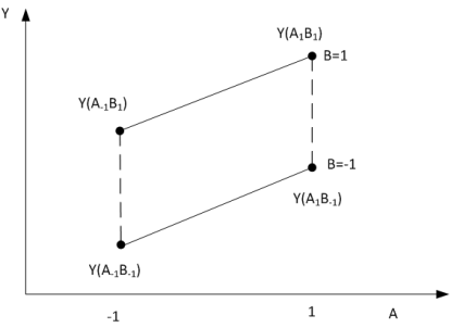
From here we can see that the effect of AB is half of the difference of the effect of B when A is fixed at 1 and the effect of B when A is fixed at -1. Therefore, a two-way interaction effect is calculated using 4 points as shown in the above equation. This is illustrated in the following figure.
As we discussed before, a main effect is defined by two points. For example, the main effect of B at A=1 is defined by
and
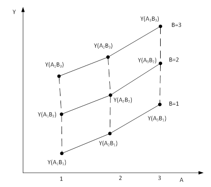
. The above figure clearly shows that a two-way interaction effect of two-level factors is defined by the 4 vertex of a quadrilateral. How can we define the two-way interaction effects of factorials with more than two levels? For example, for the design used in the previous section, A and B are both three levels. What is the interaction effect AB? For this example, the 9 design points are shown in the following figure.
Notice that there are 9 quadrilaterals in the above figure. These 9 contrasts define the interaction effect AB. This is similar to the paired comparisons in a one factorial design with multiple levels, where a main effect is defined by a group of contrasts (or paired comparisons). For the design in the above figure, to construct a quadrilateral, we need to choose 2 levels from A and 2 levels from B. There are
combinations. Therefore, we see the following 9 contrasts.
-
Contrast ID A B 1 (1, 2) (1, 2) 2 (1, 2) (1, 3) 3 (1, 2) (2, 3) 4 (1, 3) (1, 2) 5 (1, 3) (1, 3) 6 (1, 3) (2, 3) 7 (2, 3) (1, 2) 8 (2, 3) (1, 3) 9 (2, 3) (2, 3)
Let's use the first contrast to explain the meaning of a contrast. (1, 2) in column A means the selected levels from A are 1 and 2. (1, 2) in column B means the selected levels from B are 1 and 2. They form 4 points:
,
,
and
. We can denote the AB effect defined by this contrast as
.
In general, if a contrast is defined by A (i, j) and B(i', j'), then the effect is calculated by:
From the above two equations we can see that the two-way interaction effect AB is defined as the difference of the main effect of B at A = i and the main effect of B at A = j. This logic can be easily extended to three-way interactions. For example ABC can be defined as the difference of AB at C=k and AC at C=k'. Its calculation is:
For a design with A, B, and C with 3 levels, there are
contrast for the three-way interaction ABC.
Similarly, the above method can be extended for higher order interactions. By now, we know the main effect and interactions for multiple level factorial designs are defined by a group of contrasts. We will discuss how the power of these effects is calculated in the following section.
The power for an effect is defined as follows: when the largest value of a contrast group for an effect is
, power is the smallest probability of detecting this
among all the possible outcomes at a given significance level.
To calculate the power for an effect, as in the previous sections, we need to relate a contrast with model coefficients. The 9 contrasts in the above table can be expressed using model coefficients. For example:
If this contrast has the largest value
, the power is calculated from the following optimization problem:
where
, and
is the variance and covariance matrix of
.
For a balanced general level factorial design such as this example, the optimal solution for the above optimization issue is:
For all the 9 contrasts, by assuming each of the contrasts has the largest value
one by one, we can get 9 optimal solutions and 9 non-centrality parameters
. The power for the interaction effect AB is calculated using the min(
). The 9 optimal solutions are:
-
Contrast ID A B 1 (1, 2) (1, 2) 0.5 -0.5 -0.5 0.5 2 (1, 2) (1, 3) 0.5 0 -0.5 0 3 (1, 2) (2, 3) 0 0.5 0 -0.5 4 (1, 3) (1, 2) 0.5 -0.5 0 0 5 (1, 3) (1, 3) 0.5 0 0 0 6 (1, 3) (2, 3) 0 0.5 0 0 7 (2, 3) (1, 2) 0 0 0.5 -0.5 8 (2, 3) (1, 3) 0 0 0.5 0 9 (2, 3) (2, 3) 0 0 0 0.5
In the regression equation for this example, there are 4 terms for AB effect. Therefore there are 4 independent contrasts in the above table. These are contrasts 5, 6, 8, and 9. The rest of the contrasts are linear combinations of these 4 contrasts. Based on the calculation in the main effect section, we know that the standard variance matrix
for all the coefficients is:
-
I A[1] A[2] B[1] B[2] A[1]B[1] A[1]B[2] A[2]B[1] A[2]B[2] 0.0370 0 0 0 0 0 0 0 0 0 0.0741 -0.0370 0 0 0 0 0 0 0 -0.0370 0.0741 0 0 0 0 0 0 0 0 0 0.0741 -0.0370 0 0 0 0 0 0 0 -0.0370 0.0741 0 0 0 0 0 0 0 0 0 0.1481 -0.0741 -0.0741 0.0370 0 0 0 0 0 -0.0741 0.1481 0.0370 -0.0741 0 0 0 0 0 -0.0741 0.0370 0.1481 -0.0741 0 0 0 0 0 0.0370 -0.0741 -0.0741 0.1481
The variance and covariance matrix
of AB is:
Then its inverse matrix
is:
Assuming that the
we are interested in is
, then the calculated non-centrality parameters for all the contrasts are the diagonal elements of the following matrix.
=
-
3.0003 1.5002 -1.5002 1.5002 0.7501 -0.7501 -1.5002 -0.7501 0.7501 1.5002 3.0003 1.5002 0.7501 1.5002 0.7501 -0.7501 -1.5002 -0.7501 1.5002 1.5002 3.0003 -0.7501 0.7501 1.5002 0.7501 -0.7501 -1.5002 1.5002 0.7501 -0.7501 3.0003 1.5002 -1.5002 1.5002 0.7501 -0.7501 0.7501 1.5002 0.7501 1.5002 3.0064 1.5062 0.7501 1.5062 0.7562 0.7501 0.7501 1.5002 -1.5002 1.5062 3.0064 -0.7501 0.7562 1.5062 1.5002 -0.7501 0.7501 1.5002 0.7501 -0.7501 3.0003 1.5002 -1.5002 0.7501 -1.5002 -0.7501 0.7501 1.5062 0.7562 1.5002 3.0064 1.5062 0.7501 -0.7501 -1.5002 -0.7501 0.7562 1.5062 -1.5002 1.5062 3.0064
The power is calculated using the smallest value at the diagonal of the above matrix (i.e., 3.0003). The critical value for the F test is:
Please notice that for the F distribution, the first degree of freedom is 4 (the number of terms for effect AB in the regression model) and the 2nd degree of freedom is 18 (the degree of freedom of error).
The power for AB is:
If the
we are interested in is 2
, then the non-centrality parameter will be 12.0012. The power for main effect A is:
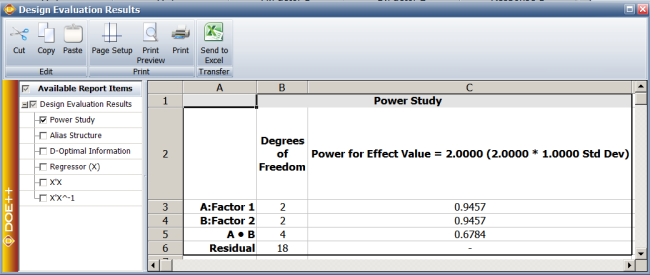
The power values for all the effects in the model are:
For balanced designs, the above calculation gives the exact power. For unbalanced design, the above method will give the approximated power. The true power is always less than the approximated value.
This section explained how to use a group of contrasts to represent the main and interaction effects for multiple level factorial designs. Examples for main and 2nd order interactions were provided. The power calculation for higher order interactions is the same as the above example. Therefore, it is not repeated here.
Power Study for Response Surface Method Designs
For response surface method designs, the following linear regression model is used:
The above equations can have both qualitative and quantitative factors. As we discussed before, for each effect (main or quadratic effect) of a quantitative factor, there is only one term in the regression model. Therefore, the power calculation for a quantitative factor is the same as treating this factor as a 2 level factor, no matter how many levels are defined for it. If qualitative factors are used in the design, they do not have quadratic effects in the model. The power calculation for qualitative factors is the same as discussed in the previous sections.
First we need to define what the "effect" is for each term in the above linear regression equation. The definition for main effects and interaction effects is the same as for 2 level factorial designs. The effect is defined as the difference of the average response at the +1 of the term and at the -1 of the term. For example, the main effect of
is:
The interaction effect of
is:
For a quadratic term
, its range is from 0 to 1. Therefore, its effect is:
The quadratic term also can be thought of as:
Since there are no grouped contrasts for each effect, the power can be calculated using either the non-central t distribution or the non-central F distribution. They will lead to the same results. Let's use the following design to illustrate the calculation.
-
Run Block A B C 1 1 -1 -1 -1 2 1 1 -1 -1 3 1 -1 1 -1 4 1 1 1 -1 5 1 -1 -1 1 6 1 1 -1 1 7 1 -1 1 1 8 1 1 1 1 9 1 0 0 0 10 1 0 0 0 11 1 0 0 0 12 1 0 0 0 13 2 -1.68179 0 0 14 2 1.681793 0 0 15 2 0 -1.68179 0 16 2 0 1.681793 0 17 2 0 0 -1.68179 18 2 0 0 1.681793 19 2 0 0 0 20 2 0 0 0 21 3 -1 -1 -1 22 3 1 -1 -1 23 3 -1 1 -1 24 3 1 1 -1 25 3 -1 -1 1 26 3 1 -1 1 27 3 -1 1 1 28 3 1 1 1 29 3 0 0 0 30 3 0 0 0 31 3 0 0 0 32 3 0 0 0 33 4 -1.68179 0 0 34 4 1.681793 0 0 35 4 0 -1.68179 0 36 4 0 1.681793 0 37 4 0 0 -1.68179 38 4 0 0 1.681793 39 4 0 0 0 40 4 0 0 0
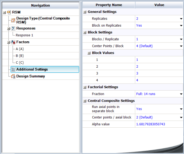
The above design can be created in a DOE folio using the following settings:
The model used here is:
Blocks are included in the model. Since there are four blocks, three indicator variables are used. The standard variance and covariance matrix
is
-
Const BLK1 BLK2 BLK3 A B C AB AC BC AA BB CC 0.085018 -0.00694 0.006944 -0.00694 0 0 0 0 0 0 -0.02862 -0.02862 -0.02862 0.00694 0.067759 -0.02609 -0.01557 0 0 0 0 0 0 0.000843 0.000843 0.000843 0.006944 -0.02609 0.088593 -0.02609 0 0 0 0 0 0 -0.00084 -0.00084 -0.00084 0.00694 -0.01557 -0.02609 0.067759 0 0 0 0 0 0 0.000843 0.000843 0.000843 0 0 0 0 0.036612 0 0 0 0 0 0 0 0 0 0 0 0 0 0.036612 0 0 0 0 0 0 0 0 0 0 0 0 0 0.036612 0 0 0 0 0 0 0 0 0 0 0 0 0 0.0625 0 0 0 0 0 0 0 0 0 0 0 0 0 0.0625 0 0 0 0 0 0 0 0 0 0 0 0 0 0.0625 0 0 0 0.02862 0.000843 -0.00084 0.000843 0 0 0 0 0 0 0.034722 0.003472 0.003472 0.02862 0.000843 -0.00084 0.000843 0 0 0 0 0 0 0.003472 0.034722 0.003472
The variances for all the coefficients are the diagonal elements in the above matrix. These are:
-
Term Var( )
A 0.036612 B 0.036612 C 0.036612 AB 0.0625 AC 0.0625 BC 0.0625 AA 0.034722 BB 0.034722 CC 0.034722
Assume the value for each effect we are interested in is
. Then, to get this
the corresponding value for each model coefficient is:
-
Term Coefficient A 0.5 B 0.5 C 0.5 AB 0.5 AC 0.5 BC 0.5 AA 1 BB 1 CC 1
The degrees of freedom used in the calculation are:
-
Source Degree of Freedom Block 3 A:A 1 B:B 1 C:C 1 AB 1 AC 1 BC 1 AA 1 BB 1 CC 1 Residual 27 Lack of Fit 19 Pure Error 8 Total 39
The above table shows all the factor effects have the same degree of freedom, therefore they have the same critical F value. For a significance level of 0.05, the critical value is:
When
, the non-centrality parameter for each main effect is calculated by:
The non-centrality parameter for each interaction effect is calculated by:
The non-centrality parameter for each quadratic effect is calculated by:
All the non-centrality parameters are given in the following table:
-
Term Non-centrality parameter ( )
A 6.828362 B 6.828362 C 6.828362 AB 4 AC 4 BC 4 AA 28.80018 BB 28.80018 CC 28.80018
The power for each term is calculated by:
They are:
-
Source Power ( )
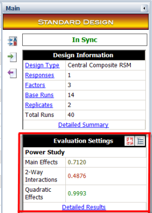
A:A 0.712033 B:B 0.712033 C:C 0.712033 AB 0.487574 AC 0.487574 BC 0.487574 AA 0.999331 BB 0.999331 CC 0.999331
The results in a DOE folio can be obtained from the design evaluation.
Discussion on Power Calculation
All the above examples show how to calculate the power for a given amount of effect. When a power value is given, using the above method we also can calculate the corresponding effect. If the power is too low for an effect of interest, the sample size of the experiment must be increased in order to get a higher power value.
We discussed in detail how to define an "effect" for quantitative and qualitative factors, and how to use model coefficients to represent a given effect. The power in a DOE folio is calculated based on this definition. Readers may find that power is calculated directly based on model coefficients (instead of the contrasts) in other software packages or books. However, for some cases, such as for the main and interaction effects of qualitative factors with multiple levels, the meaning of model coefficients is not very straightforward. Therefore, it is better to use the defined effect (or contrast) shown here to calculate the power, even though this calculation is much more complicated.
Conclusion
In this chapter, we discussed how to evaluate an experiment design. Although the evaluation can be conducted either before or after conducting the experiment, it is always recommended to evaluate an experiment before performing it. A bad design will waste time and money. Readers should check the alias structure, the orthogonality and the power for important effects for an experiment before the tests.


![{\displaystyle {\begin{aligned}&E\left({{\hat {\beta }}_{1}}\right)=E\left[{{\left(X_{1}^{'}{{X}_{1}}\right)}^{-1}}X_{1}^{'}Y\right]\\&={{\left(X_{1}^{'}{{X}_{1}}\right)}^{-1}}X_{1}^{'}E(Y)\\&={{\left(X_{1}^{'}{{X}_{1}}\right)}^{-1}}X_{1}^{'}E({{X}_{1}}{{\beta }_{1}}+{{X}_{2}}{{\beta }_{2}}+\varepsilon )\\&={{\left(X_{1}^{'}{{X}_{1}}\right)}^{-1}}X_{1}^{'}{{X}_{1}}{{\beta }_{1}}+{{\left(X_{1}^{'}{{X}_{1}}\right)}^{-1}}X_{1}^{'}{{X}_{2}}{{\beta }_{2}}\\&={{\beta }_{1}}+A{{\beta }_{2}}\end{aligned}}\,\!}](https://en.wikipedia.org/api/rest_v1/media/math/render/svg/42de5775c8d1b642793b9351eb1f605fd8c81111)


![{\displaystyle {{X}_{1}}=[I{\text{ }}A{\text{ }}B{\text{ }}C]\,\!}](https://en.wikipedia.org/api/rest_v1/media/math/render/svg/e613f4c55ce1344ebbd6df2183d352b67c4e4e2e)
![{\displaystyle {{X}_{2}}=[AB{\text{ }}AC{\text{ }}BC{\text{ }}ABC]\,\!}](https://en.wikipedia.org/api/rest_v1/media/math/render/svg/d49e5e847f86f5cb76e0f92d557b615063dfb7a0)

![{\displaystyle {\begin{aligned}&[I]=I+ABC\\&[A]=A+BC\\&[B]=B+AC\\&[C]=C+AB\\\end{aligned}}\,\!}](https://en.wikipedia.org/api/rest_v1/media/math/render/svg/e4f1e565a116a6fccb149a1b62b4e5367e309008)






![{\displaystyle \min {\text{ }}\phi {\text{=}}{\frac {{\text{2}}n}{{\sigma }^{2}}}\left[\sum \limits _{i=1}^{r}{\beta _{i}^{2}}+\sum \limits _{i=1}^{r}{\sum \limits _{i\neq j}^{r}{{{\beta }_{i}}{{\beta }_{j}}}}\right]\,\!}](https://en.wikipedia.org/api/rest_v1/media/math/render/svg/90ddd809ed631c8b4f8d65039f38cdec10f63019)


![{\displaystyle \phi {\text{=}}{\frac {{\text{2}}n}{{\sigma }^{2}}}\left[\sum \limits _{i=1}^{r}{\beta _{i}^{2}}+\sum \limits _{i=1}^{r}{\sum \limits _{i\neq j}^{r}{{{\beta }_{i}}{{\beta }_{j}}}}\right]\,\!}](https://en.wikipedia.org/api/rest_v1/media/math/render/svg/7b541abb27f977e1060f6058cf66125099d7db68)



![{\displaystyle {\begin{aligned}&Y={{\beta }_{0}}+{{\beta }_{1}}A[1]+{{\beta }_{2}}A[2]+{{\beta }_{3}}B[1]+{{\beta }_{4}}B[2]+{{\beta }_{11}}A[1]B[1]\\&+{{\beta }_{12}}A[1]B[2]+{{\beta }_{21}}A[2]B[1]+{{\beta }_{22}}A[2]B[2]\end{aligned}}\,\!}](https://en.wikipedia.org/api/rest_v1/media/math/render/svg/e61b08aca6711b127dacf43ac215a015b863d305)











![{\displaystyle {\begin{aligned}&Y={{\beta }_{0}}+{{\beta }_{b1}}BLK[1]+{{\beta }_{b2}}BLK[2]+{{\beta }_{b3}}BLK[3]+{{\beta }_{1}}A+{{\beta }_{2}}B+{{\beta }_{3}}C\\&+{{\beta }_{12}}AB+{{\beta }_{13}}AC+{{\beta }_{23}}BC+{{\beta }_{11}}{{A}^{2}}+{{\beta }_{22}}{{B}^{2}}+{{\beta }_{33}}{{C}^{2}}\end{aligned}}\,\!}](https://en.wikipedia.org/api/rest_v1/media/math/render/svg/ae49c9fdd9f7ffb112e4d74aae646a74ea415269)


