Temperature-NonThermal Relationship
When temperature and a second non-thermal stress (e.g., voltage) are the accelerated stresses of a test, then the Arrhenius and the inverse power law relationships can be combined to yield the Temperature-NonThermal (T-NT) relationship. This relationship is given by:
where:
is the non-thermal stress (i.e., voltage, vibration, etc.)
is the temperature (in absolute units).
,
,
are the parameters to be determined.
The T-NT relationship can be linearized and plotted on a Life vs. Stress plot. The relationship is linearized by taking the natural logarithm of both sides in the T-NT relationship or:
Since life is now a function of two stresses, a Life vs. Stress plot can only be obtained by keeping one of the two stresses constant and varying the other one. Doing so will yield the straight line described by the above equation, where the term for the stress which is kept at a fixed value becomes another constant (in addition to the
constant).
When the non-thermal stress is kept constant, then the linearized T-NT relationship becomes:
This is the Arrhenius equation and it is plotted on a log-reciprocal scale. When the thermal stress is kept constant, then the linearized T-NT relationship becomes:
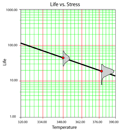
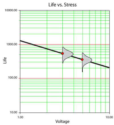
This is the inverse power law equation and it is plotted on a log-log scale. In the next two figures, data obtained from a temperature and voltage test were analyzed and plotted on a log-reciprocal scale. In the first figure, life is plotted versus temperature, with voltage held at a fixed value. In the second figure, life is plotted versus voltage, with temperature held at a fixed value.
A look at the Parameters B and n
Depending on which stress type is kept constant, it can be seen from the linearized T-NT relationship that either the parameter
or the parameter
is the slope of the resulting line. If, for example, the non-thermal stress is kept constant then
is the slope of the life line in a Life vs. Temperature plot. The steeper the slope, the greater the dependency of the product's life to the temperature. In other words,
is a measure of the effect that temperature has on the life and
is a measure of the effect that the non-thermal stress has on the life. The larger the value of
the higher the dependency of the life on the temperature. Similarly, the larger the value of
the higher the dependency of the life on the non-thermal stress.
Acceleration Factor
The acceleration factor for the T-NT relationship is given by:
where:
is the life at use stress level.
is the life at the accelerated stress level.
is the use temperature level.
is the accelerated temperature level.
is the accelerated non-thermal level.
is the use non-thermal level.
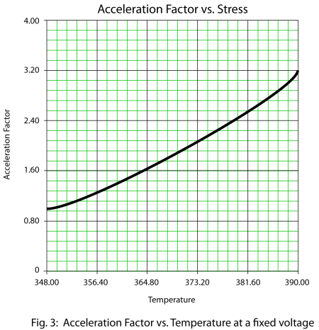
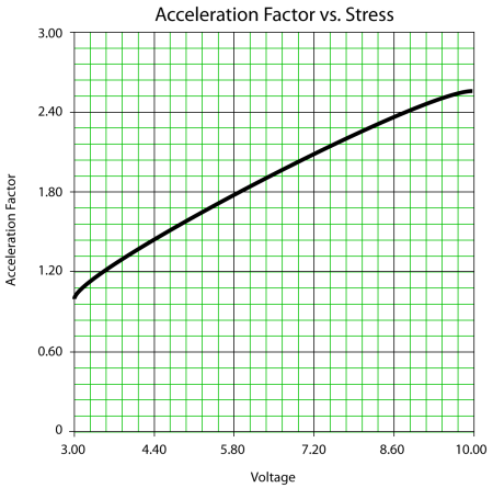
The acceleration factor is plotted versus stress in the same manner used to create the Life vs. Stress plots. That is, one stress type is kept constant and the other is varied.
T-NT Exponential
By setting , the exponential
pdf becomes:
T-NT Exponential Statistical Properties Summary
Mean or MTTF
The mean, or Mean Time To Failure (MTTF) for the T-NT exponential model is given by:
Median
The median, for the T-NT exponential model is given by:
Mode
The mode, for the T-NT exponential model is given by:
Standard Deviation
The standard deviation, , for the T-NT exponential model is given by:
T-NT Exponential Reliability Function
The T-NT exponential reliability function is given by:
This function is the complement of the T-NT exponential cumulative distribution function or:
and,
Conditional Reliability
The conditional reliability function for the T-NT exponential model is given by,
Reliable Life
For the T-NT exponential model, the reliable life, or the mission duration for a desired reliability goal,
, is given by:
- or:
Parameter Estimation
Maximum Likelihood Estimation Method
Substituting the T-NT relationship into the exponential log-likelihood equation yields:
where:
and:
is the number of groups of exact times-to-failure data points.
is the number of times-to-failure data points in the
time-to-failure data group.
is the T-NT parameter (unknown, the first of three parameters to be estimated).
is the second T-NT parameter (unknown, the second of three parameters to be estimated).
is the third T-NT parameter (unknown, the third of three parameters to be estimated).
is the temperature level of the
group.
is the non-thermal stress level of the
group.
is the exact failure time of the
group.
is the number of groups of suspension data points.
is the number of suspensions in the
group of suspension data points.
is the running time of the
suspension data group.
is the number of interval data groups.
is the number of intervals in the
group of data intervals.
is the beginning of the
interval.
is the ending of the
interval.
The solution (parameter estimates) will be found by solving for the parameters
and
so that
and
.
T-NT Weibull
By setting , the T-NT Weibull model is given by:
T-NT Weibull Statistical Properties Summary
Mean or MTTF
The mean, , for the T-NT Weibull model is given by:
where is the gamma function evaluated at the value of
.
Median
The median, for the T-NT Weibull model is given by:
Mode
The mode, for the T-NT Weibull model is given by:
Standard Deviation
The standard deviation, for the T-NT Weibull model is given by:
T-NT Weibull Reliability Function
The T-NT Weibull reliability function is given by:
Conditional Reliability Function
The T-NT Weibull conditional reliability function at a specified stress level is given by:
or:
Reliable Life
For the T-NT Weibull model, the reliable life,
, of a unit for a specified reliability and starting the mission at age zero is given by:
T-NT Weibull Failure Rate Function
The T-NT Weibull failure rate function,
, is given by:
Parameter Estimation
Maximum Likelihood Estimation Method
Substituting the T-NT relationship into the Weibull log-likelihood function yields:
where:
and:
is the number of groups of exact times-to-failure data points.
is the number of times-to-failure data points in the
time-to-failure data group.
is the Weibull shape parameter (unknown, the first of four parameters to be estimated).
is the first T-NT parameter (unknown, the second of four parameters to be estimated).
is the second T-NT parameter (unknown, the third of four parameters to be estimated).
is the third T-NT parameter (unknown, the fourth of four parameters to be estimated).
is the temperature level of the
group.
is the non-thermal stress level of the
group.
is the exact failure time of the
group.
is the number of groups of suspension data points.
is the number of suspensions in the
group of suspension data points.
is the running time of the
suspension data group.
is the number of interval data groups.
is the number of intervals in the
group of data intervals.
is the beginning of the
interval.
is the ending of the
interval.
The solution (parameter estimates) will be found by solving for the parameters
and
so that
and
.
T-NT Lognormal
The pdf of the lognormal distribution is given by:
where:
and:
times-to-failure.
mean of the natural logarithms of the times-to-failure.
standard deviation of the natural logarithms of the times-to-failure.
The median of the lognormal distribution is given by:
The T-NT lognormal model pdf can be obtained by setting
. Therefore:
or:
Thus:
Substituting the above equation into the lognormal pdf yields the T-NT lognormal model pdf or:
T-N-T Lognormal Statistical Properties Summary
The Mean
The mean life of the T-NT lognormal model (mean of the times-to-failure),
, is given by:
The mean of the natural logarithms of the times-to-failure,
, in terms of
and
is given by:
The Standard Deviation
The standard deviation of the T-NT lognormal model (standard deviation of the times-to-failure),
, is given by:
The standard deviation of the natural logarithms of the times-to-failure,
, in terms of
and
is given by:
The Mode
The mode of the T-NT lognormal model is given by:
T-NT Lognormal Reliability
For the T-NT lognormal model, the reliability for a mission of time
, starting at age 0, for the T-NT lognormal model is determined by:
or:
Reliable Life
For the T-NT lognormal model, the reliable life, or the mission duration for a desired reliability goal,
is estimated by first solving the reliability equation with respect to time, as follows:
where:
and:
Since the reliable life,
, is given by:
Lognormal Failure Rate
The T-NT lognormal failure rate is given by:
Parameter Estimation
Maximum Likelihood Estimation Method
The complete T-NT lognormal log-likelihood function is:
where:
and:
is the number of groups of exact times-to-failure data points.
is the number of times-to-failure data points in the
time-to-failure data group.
is the standard deviation of the natural logarithm of the times-to-failure (unknown, the first of four parameters to be estimated).
is the first T-NT parameter (unknown, the second of four parameters to be estimated).
is the second T-NT parameter (unknown, the third of four parameters to be estimated).
is the third T-NT parameter (unknown, the fourth of four parameters to be estimated).
is the stress level for the first stress type (i.e., temperature) of the
group.
is the stress level for the second stress type (i.e., non-thermal) of the
group.
is the exact failure time of the
group.
is the number of groups of suspension data points.
is the number of suspensions in the
group of suspension data points.
is the running time of the
suspension data group.
is the number of interval data groups.
is the number of intervals in the
group of data intervals.
is the beginning of the
interval.
is the ending of the
interval.
The solution (parameter estimates) will be found by solving for
so that
and
.
T-NT Lognormal Example
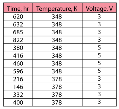
12 electronic devices were put into a continuous accelerated life test and the following data were collected.
Using Weibull++ and the T-NT lognormal model, the following parameters were obtained:
A probability plot, with the 2-sided 90% confidence bounds for the use stress levels of 323K and 2V, is shown next.
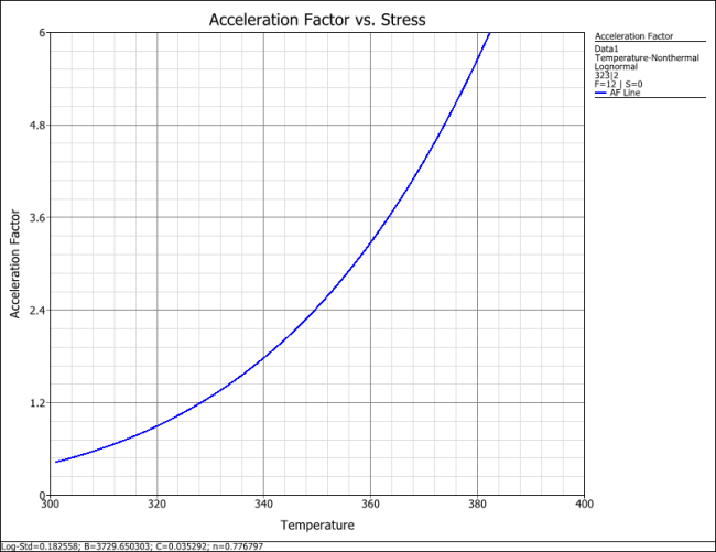
An acceleration factor plot, in which one of the stresses must be kept constant, can also be obtained. For example, in the following plot, the acceleration factor is plotted versus temperature given a constant voltage of 2V.
T-NT Confidence Bounds
Approximate Confidence Bounds for the T-NT Exponential
Confidence Bounds on the Mean Life
The mean life for the T-NT model is given by setting
. The upper
and lower
bounds on the mean life (ML estimate of the mean life) are estimated by:
where is defined by:
If is the confidence level, then
for the two-sided bounds, and
for the one-sided bounds. The variance of
is given by:
or:
The variances and covariance of and
are estimated from the local Fisher matrix (evaluated at
as follows:
where:
Confidence Bounds on Reliability
The bounds on reliability at a given time,
, are estimated by:
Confidence Bounds on Time
The bounds on time for a given reliability (ML estimate of time) are estimated by first solving the reliability function with respect to time:
The corresponding confidence bounds are estimated from:
Approximate Confidence Bounds for the T-NT Weibull
Bounds on the Parameters
Using the same approach as previously discussed (
and
positive parameters):
and:
The variances and covariances of and
are estimated from the Fisher matrix (evaluated at
as follows:
where:
Confidence Bounds on Reliability
The reliability function (ML estimate) for the T-NT Weibull model is given by:
or:
Setting:
or:
The reliability function now becomes:
The next step is to find the upper and lower bounds on
:
where:
or:
The upper and lower bounds on reliability are:
Confidence Bounds on Time
The bounds on time (ML estimate of time) for a given reliability are estimated by first solving the reliability function with respect to time as follows:
or:
where
The upper and lower bounds on are estimated from:
where:
or:
The upper and lower bounds on time are then found by:
Approximate Confidence Bounds for the T-NT Lognormal
Bounds on the Parameters
Since the standard deviation, , and
are positive parameters,
and
are treated as normally distributed and the bounds are estimated from:
and:
The lower and upper bounds on and
are estimated from:
and:
The variances and covariances of ,
and
are estimated from the local Fisher matrix (evaluated at
,
as follows:
- where:
Bounds on Reliability
The reliability of the lognormal distribution is given by:
Let then
For
,
, and for
The above equation then becomes:
The bounds on are estimated from:
where:
or:
The upper and lower bounds on reliability are:
Confidence Bounds on Time
The bounds around time for a given lognormal percentile (unreliability) are estimated by first solving the reliability equation with respect to time, as follows:
where:
and:
The next step is to calculate the variance of
:
or:
The upper and lower bounds are then found by:
Solving for and
yields:






![{\displaystyle \ln[R({{t}_{R}},U,V)]{{=}^{-{\tfrac {{{t}_{R}}\cdot {{U}^{n}}{{e}^{-{\tfrac {B}{V}}}}}{C}}}}\,\!}](https://en.wikipedia.org/api/rest_v1/media/math/render/svg/d89e07341cef26276e1da4708fe0731829d1b52b)
![{\displaystyle {{t}_{R}}=-{\frac {C}{{{U}^{n}}{{e}^{-{\tfrac {B}{V}}}}}}\ln[R({{t}_{R}},U,V)]\,\!}](https://en.wikipedia.org/api/rest_v1/media/math/render/svg/0e2f4d089e2fc97016d5b5b97bad5009f7386fde)
![{\displaystyle {\begin{aligned}&\ln(L)=&\Lambda ={\underset {i=1}{\overset {{F}_{e}}{\mathop {\sum } }}}\,{{N}_{i}}\ln \left[{\frac {U_{i}^{n}}{C}}{{e}^{-{\tfrac {B}{{V}_{i}}}}}\cdot {{e}^{-{\tfrac {U_{i}^{n}}{C}}\left({{e}^{-{\tfrac {B}{{V}_{i}}}}}\right){{T}_{i}}}}\right]-{\underset {i=1}{\overset {S}{\mathop {\sum } }}}\,N_{i}^{\prime }{\frac {U_{i}^{n}}{C}}\left({{e}^{-{\tfrac {B}{{V}_{i}}}}}\right)T_{i}^{\prime }+{\overset {FI}{\mathop {{\underset {i=1}{\mathop {{\underset {}{\overset {}{\mathop {\sum } }}}\,} }}\,} }}\,N_{i}^{\prime \prime }\ln[R_{Li}^{\prime \prime }-R_{Ri}^{\prime \prime }]\end{aligned}}\,\!}](https://en.wikipedia.org/api/rest_v1/media/math/render/svg/01d1885576883e9cac66e9808e5d9356d472c472)


![{\displaystyle R((t|T),U,V)={{e}^{-\left[{{\left({\tfrac {\left(T+t\right){{U}^{n}}{{e}^{-{\tfrac {B}{V}}}}}{C}}\right)}^{\beta }}-{{\left({\tfrac {T{{U}^{n}}{{e}^{-{\tfrac {B}{V}}}}}{C}}\right)}^{\beta }}\right]}}\,\!}](https://en.wikipedia.org/api/rest_v1/media/math/render/svg/d85ec527575321251bbb34005148355889fa5911)

![{\displaystyle {{T}_{R}}={\frac {C}{{{U}^{n}}{{e}^{-{\tfrac {B}{V}}}}}}{{\left\{-\ln \left[R\left({{T}_{R}},U,V\right)\right]\right\}}^{\tfrac {1}{\beta }}}\,\!}](https://en.wikipedia.org/api/rest_v1/media/math/render/svg/aa257921e416fb3d96de2c121da1a9210f3f5afc)


![{\displaystyle {\begin{aligned}&\ln(L)=&\Lambda ={\underset {i=1}{\overset {{F}_{e}}{\mathop {\sum } }}}\,{{N}_{i}}\ln \left[{\frac {\beta U_{i}^{n}{{e}^{-{\tfrac {B}{{V}_{i}}}}}}{C}}{{\left({\frac {U_{i}^{n}{{e}^{-{\tfrac {B}{{V}_{i}}}}}}{C}}{{T}_{i}}\right)}^{\beta -1}}{{e}^{-{{\left({\tfrac {U_{i}^{n}{{e}^{-{\tfrac {B}{{V}_{i}}}}}}{C}}{{T}_{i}}\right)}^{\beta }}}}\right]-{\underset {i=1}{\overset {S}{\mathop {\sum } }}}\,N_{i}^{\prime }{{\left({\frac {U_{i}^{n}{{e}^{-{\tfrac {B}{{V}_{i}}}}}}{C}}T_{i}^{\prime }\right)}^{\beta }}+{\overset {FI}{\mathop {{\underset {i=1}{\mathop {{\underset {}{\overset {}{\mathop {\sum } }}}\,} }}\,} }}\,N_{i}^{\prime \prime }\ln[R_{Li}^{\prime \prime }-R_{Ri}^{\prime \prime }]\end{aligned}}\,\!}](https://en.wikipedia.org/api/rest_v1/media/math/render/svg/422992549c4c64a28a6eb7faeda45a9adcd955a3)


![{\displaystyle z={{\Phi }^{-1}}\left[F\left(T_{R}^{\prime },U,V\right)\right]\,\!}](https://en.wikipedia.org/api/rest_v1/media/math/render/svg/9de498105ad0dee66fb24643bb1c421c6a139cc3)


![{\displaystyle {\begin{aligned}&\ln(L)=&\Lambda ={\underset {i=1}{\overset {{F}_{e}}{\mathop {\sum } }}}\,{{N}_{i}}\ln \left[{\frac {1}{{{\sigma }_{{T}'}}{{T}_{i}}}}{{\phi }_{pdf}}\left({\frac {\ln \left({{T}_{i}}\right)-\ln(C)+n\ln({{U}_{i}})-{\tfrac {B}{{V}_{i}}}}{{\sigma }_{{T}'}}}\right)\right]{\text{ }}+{\underset {i=1}{\overset {S}{\mathop {\sum } }}}\,N_{i}^{\prime }\ln \left[1-\Phi \left({\frac {\ln \left(T_{i}^{\prime }\right)-\ln(C)+n\ln({{U}_{i}})-{\tfrac {B}{{V}_{i}}}}{{\sigma }_{{T}'}}}\right)\right]+{\overset {FI}{\mathop {{\underset {i=1}{\mathop {{\underset {}{\overset {}{\mathop {\sum } }}}\,} }}\,} }}\,N_{i}^{\prime \prime }\ln[\Phi (z_{Ri}^{\prime \prime })-\Phi (z_{Li}^{\prime \prime })]\end{aligned}}\,\!}](https://en.wikipedia.org/api/rest_v1/media/math/render/svg/3395e305993ddc31cae339b41e1ed1522d761f82)






![{\displaystyle {\begin{aligned}Var({\widehat {m}})=&{\frac {1}{{U}^{2{\widehat {n}}}}}{{e}^{2{\tfrac {\widehat {B}}{V}}}}[{\frac {{\widehat {C}}^{2}}{{V}^{2}}}Var({\widehat {B}})+Var({\widehat {C}})+{{\widehat {C}}^{2}}{{\left(\ln(U)\right)}^{2}}Var({\widehat {n}})+{\frac {2{\widehat {C}}}{V}}Cov({\widehat {B}},{\widehat {C}})\\&-{\frac {2{{\widehat {C}}^{2}}\ln(U)}{V}}Cov({\widehat {B}},{\widehat {n}})-2{\widehat {C}}\ln(U)Cov({\widehat {C}},{\widehat {n}})]\end{aligned}}\,\!}](https://en.wikipedia.org/api/rest_v1/media/math/render/svg/46915cfc06a025e1b06eeb862002eff792877c7b)

![{\displaystyle \left[{\begin{matrix}Var({\widehat {B}})&Cov({\widehat {B}},{\widehat {C}})&Cov({\widehat {B}},{\widehat {n}})\\Cov({\widehat {C}},{\widehat {B}})&Var({\widehat {C}})&Cov({\widehat {C}},{\widehat {n}})\\Cov({\widehat {n}},{\widehat {B}})&Cov({\widehat {n}},{\widehat {C}})&Var({\widehat {n}})\\\end{matrix}}\right]={{\left[F\right]}^{-1}}\,\!}](https://en.wikipedia.org/api/rest_v1/media/math/render/svg/c1005375d89f8cfcdb4151220f910aea1e6f00ae)
![{\displaystyle F=\left[{\begin{matrix}-{\tfrac {{{\partial }^{2}}\Lambda }{\partial {{B}^{2}}}}&-{\tfrac {{{\partial }^{2}}\Lambda }{\partial B\partial C}}&-{\tfrac {{{\partial }^{2}}\Lambda }{\partial B\partial n}}\\-{\tfrac {{{\partial }^{2}}\Lambda }{\partial C\partial B}}&-{\tfrac {{{\partial }^{2}}\Lambda }{\partial {{C}^{2}}}}&-{\tfrac {{{\partial }^{2}}\Lambda }{\partial C\partial n}}\\-{\tfrac {{{\partial }^{2}}\Lambda }{\partial n\partial B}}&-{\tfrac {{{\partial }^{2}}\Lambda }{\partial n\partial C}}&-{\tfrac {{{\partial }^{2}}\Lambda }{\partial {{n}^{2}}}}\\\end{matrix}}\right].\,\!}](https://en.wikipedia.org/api/rest_v1/media/math/render/svg/dac079b419d54078b49816b493d6abcd18d7e4f4)


![{\displaystyle \left[{\begin{matrix}Var({\widehat {\beta }})&Cov({\widehat {\beta }},{\widehat {B}})&Cov({\widehat {\beta }},{\widehat {C}})&Cov({\widehat {\beta }},{\widehat {n}})\\Cov({\widehat {B}},{\widehat {\beta }})&Var({\widehat {B}})&Cov({\widehat {B}},{\widehat {C}})&Cov({\widehat {B}},{\widehat {n}})\\Cov({\widehat {C}},{\widehat {\beta }})&Cov({\widehat {C}},{\widehat {B}})&Var({\widehat {C}})&Cov({\widehat {C}},{\widehat {n}})\\Cov({\widehat {n}},{\widehat {\beta }})&Cov({\widehat {n}},{\widehat {B}})&Cov({\widehat {n}},{\widehat {C}})&Var({\widehat {n}})\\\end{matrix}}\right]={{\left[F\right]}^{-1}}\,\!}](https://en.wikipedia.org/api/rest_v1/media/math/render/svg/8c989e09904a1c39a32426d8d1e892eb35286c68)
![{\displaystyle F=\left[{\begin{matrix}-{\tfrac {{{\partial }^{2}}\Lambda }{\partial {{\beta }^{2}}}}&-{\tfrac {{{\partial }^{2}}\Lambda }{\partial \beta \partial B}}&-{\tfrac {{{\partial }^{2}}\Lambda }{\partial \beta \partial C}}&-{\tfrac {{{\partial }^{2}}\Lambda }{\partial \beta \partial n}}\\-{\tfrac {{{\partial }^{2}}\Lambda }{\partial B\partial \beta }}&-{\tfrac {{{\partial }^{2}}\Lambda }{\partial {{B}^{2}}}}&-{\tfrac {{{\partial }^{2}}\Lambda }{\partial B\partial C}}&-{\tfrac {{{\partial }^{2}}\Lambda }{\partial B\partial n}}\\-{\tfrac {{{\partial }^{2}}\Lambda }{\partial C\partial \beta }}&-{\tfrac {{{\partial }^{2}}\Lambda }{\partial C\partial B}}&-{\tfrac {{{\partial }^{2}}\Lambda }{\partial {{C}^{2}}}}&-{\tfrac {{{\partial }^{2}}\Lambda }{\partial C\partial n}}\\-{\tfrac {{{\partial }^{2}}\Lambda }{\partial n\partial \beta }}&-{\tfrac {{{\partial }^{2}}\Lambda }{\partial n\partial B}}&-{\tfrac {{{\partial }^{2}}\Lambda }{\partial n\partial C}}&-{\tfrac {{{\partial }^{2}}\Lambda }{\partial {{n}^{2}}}}\\\end{matrix}}\right]\,\!}](https://en.wikipedia.org/api/rest_v1/media/math/render/svg/6aa61aa2dab719065eccf58b1da9d215955f82da)

![{\displaystyle {\widehat {R}}(T,U,V)={{e}^{-{{e}^{\ln \left[{{\left({\tfrac {{{U}^{\widehat {n}}}{{e}^{-{\tfrac {\widehat {B}}{V}}}}}{\widehat {C}}}T\right)}^{\widehat {\beta }}}\right]}}}}\,\!}](https://en.wikipedia.org/api/rest_v1/media/math/render/svg/9e2fdb10158f96ee2ec8e9230e4be072309055d6)
![{\displaystyle {\widehat {u}}=\ln \left[{{\left({\frac {{{U}^{\widehat {n}}}{{e}^{-{\tfrac {\widehat {B}}{V}}}}}{\widehat {C}}}T\right)}^{\widehat {\beta }}}\right]\,\!}](https://en.wikipedia.org/api/rest_v1/media/math/render/svg/f14165533b1a5f3f0ae5526c2c26e44757540de0)
![{\displaystyle {\widehat {u}}={\widehat {\beta }}\left[\ln(T)-{\frac {\widehat {B}}{V}}-\ln({\widehat {C}})+{\widehat {n}}\ln(U)\right]\,\!}](https://en.wikipedia.org/api/rest_v1/media/math/render/svg/c979f23f83c76ec33ef36d6bf449128de033c4eb)


![{\displaystyle {\begin{aligned}Var({\widehat {u}})=&{\frac {1}{{\widehat {\beta }}^{4}}}{{\left[\ln(-\ln(R))\right]}^{2}}Var({\widehat {\beta }})+{\frac {1}{{V}^{2}}}Var({\widehat {B}})+{\frac {1}{{\widehat {C}}^{2}}}Var({\widehat {C}})+{{\left[\ln(U)\right]}^{2}}Var({\widehat {n}})-{\frac {2\ln(-\ln(R))}{{{\widehat {\beta }}^{2}}V}}Cov({\widehat {\beta }},{\widehat {B}})-{\frac {2\ln(-\ln(R))}{{{\widehat {\beta }}^{2}}{\widehat {C}}}}Cov({\widehat {\beta }},{\widehat {C}})\\&+{\frac {2\ln(-\ln(R))\ln(U)}{{\widehat {\beta }}^{2}}}Cov({\widehat {\beta }},{\widehat {n}})+{\frac {2}{{\widehat {C}}V}}Cov({\widehat {B}},{\widehat {C}})-{\frac {2\ln(U)}{V}}Cov({\widehat {B}},{\widehat {n}})-{\frac {2\ln(U)}{\widehat {C}}}Cov({\widehat {C}},{\widehat {n}})\end{aligned}}\,\!}](https://en.wikipedia.org/api/rest_v1/media/math/render/svg/998176f3c30fb74697ea3fa746d7833505b33b67)


![{\displaystyle \left({\begin{matrix}Var\left({{\widehat {\sigma }}_{{T}'}}\right)&Cov\left({\widehat {B}},{{\widehat {\sigma }}_{{T}'}}\right)&Cov\left({\widehat {C}},{{\widehat {\sigma }}_{{T}'}}\right)&Cov\left({\widehat {n}},{{\widehat {\sigma }}_{{T}'}}\right)\\Cov\left({{\widehat {\sigma }}_{{T}'}},{\widehat {B}}\right)&Var\left({\widehat {B}}\right)&Cov\left({\widehat {B}},{\widehat {C}}\right)&Cov\left({\widehat {B}},{\widehat {n}}\right)\\Cov\left({{\widehat {\sigma }}_{{T}'}},{\widehat {C}}\right)&Cov\left({\widehat {C}},{\widehat {B}}\right)&Var\left({\widehat {C}}\right)&Cov\left({\widehat {C}},{\widehat {n}}\right)\\Cov\left({\widehat {n}},{{\widehat {\sigma }}_{{T}'}}\right)&Cov\left({\widehat {n}},{\widehat {B}}\right)&Cov\left({\widehat {n}},{\widehat {C}}\right)&Var\left({\widehat {n}}\right)\\\end{matrix}}\right)={{\left[F\right]}^{-1}}\,\!}](https://en.wikipedia.org/api/rest_v1/media/math/render/svg/da4d1aa6713292d66ea9fec7b220d1ae5d051731)


![{\displaystyle {\begin{aligned}Var({\widehat {z}})=&{\frac {1}{{\widehat {\sigma }}_{{T}'}^{2}}}[{\frac {1}{{V}^{2}}}Var({\widehat {B}})+{\frac {1}{{C}^{2}}}Var({\widehat {C}})+\ln {{(U)}^{2}}Var({\widehat {n}})+{{\widehat {z}}^{2}}Var({{\widehat {\sigma }}_{{T}'}})+{\frac {2}{C\cdot V}}Cov\left({\widehat {B}},{\widehat {C}}\right)-{\frac {2\ln(U)}{V}}Cov\left({\widehat {B}},{\widehat {n}}\right)\\&-{\frac {2\ln(U)}{C}}Cov\left({\widehat {C}},{\widehat {n}}\right)+{\frac {2{\widehat {z}}}{V}}Cov\left({\widehat {B}},{{\widehat {\sigma }}_{{T}'}}\right)+{\frac {2{\widehat {z}}}{C}}Cov\left({\widehat {C}},{{\widehat {\sigma }}_{{T}'}}\right)-2{\widehat {z}}\ln(U)Cov\left({\widehat {n}},{{\widehat {\sigma }}_{{T}'}}\right)]\end{aligned}}\,\!}](https://en.wikipedia.org/api/rest_v1/media/math/render/svg/97f58f05b25de8f7bc92c31c00f428a7d217b67b)


![{\displaystyle {\begin{aligned}{T}'(U,V;{\widehat {A}},{\widehat {\phi }},{\widehat {b}},{{\widehat {\sigma }}_{{T}'}})=\ &\ln(T)\\z=\ &{{\Phi }^{-1}}\left[F({T}')\right]\end{aligned}}\,\!}](https://en.wikipedia.org/api/rest_v1/media/math/render/svg/85f49c3d5218d4bba28dbf13edcde56f5254fd86)


