Inverse Power Law Relationship
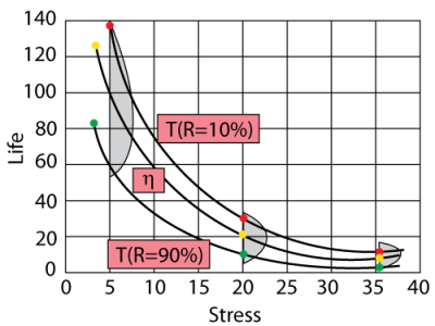
The inverse power law (IPL) model (or relationship) is commonly used for non-thermal accelerated stresses and is given by:
where:
represents a quantifiable life measure, such as mean life, characteristic life, median life,
life, etc.
represents the stress level.
is one of the model parameters to be determined,
is another model parameter to be determined.
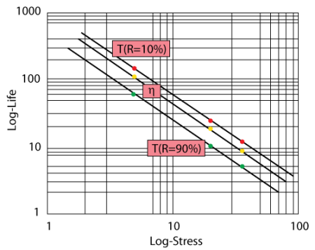
The inverse power law appears as a straight line when plotted on a log-log paper. The equation of the line is given by:
Plotting methods are widely used in estimating the parameters of the inverse power law relationship since obtaining
and
is as simple as finding the slope and the intercept in the above equation.
A Look at the Parameter n
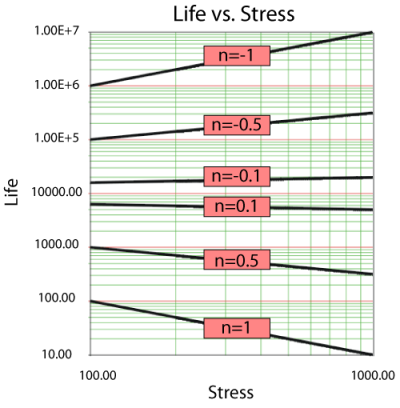
The parameter in the inverse power relationship is a measure of the effect of the stress on the life. As the absolute value of
increases, the greater the effect of the stress. Negative values of
indicate an increasing life with increasing stress. An absolute value of
approaching zero indicates small effect of the stress on the life, with no effect (constant life with stress) when
Acceleration Factor
For the IPL relationship the acceleration factor is given by:
where:
is the life at use stress level.
is the life at the accelerated stress level.
is the use stress level.
is the accelerated stress level.
IPL-Exponential
The IPL-exponential model can be derived by setting
in the exponential
pdf, yielding the following IPL-exponential pdf:
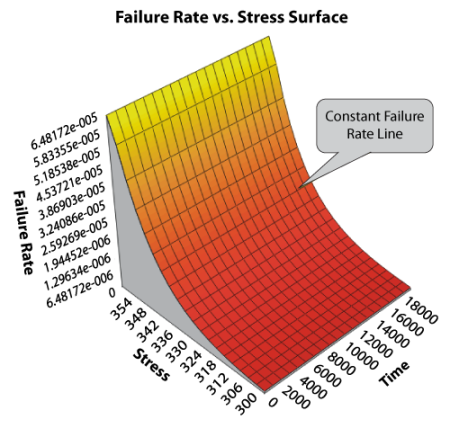
Note that this is a 2-parameter model. The failure rate (the parameter of the exponential distribution) of the model is simply
and is only a function of stress.
IPL-Exponential Statistical Properties Summary
Mean or MTTF
The mean, or Mean Time To Failure (MTTF) for the IPL-exponential relationship is given by:
Note that the MTTF is a function of stress only and is simply equal to the IPL relationship (which is the original assumption), when using the exponential distribution.
Median
The median, for the IPL-exponential model is given by:
Mode
The mode, for the IPL-exponential model is given by:
Standard Deviation
The standard deviation, , for the IPL-exponential model is given by:
IPL-Exponential Reliability Function
The IPL-exponential reliability function is given by:
This function is the complement of the IPL-exponential cumulative distribution function:
or:
Conditional Reliability
The conditional reliability function for the IPL-exponential model is given by:
Reliable Life
For the IPL-exponential model, the reliable life or the mission duration for a desired reliability goal,
is given by:
or:
Parameter Estimation
Maximum Likelihood Parameter Estimation
Substituting the inverse power law relationship into the exponential log-likelihood equation yields:
where:
and:
is the number of groups of exact times-to-failure data points.
is the number of times-to-failure in the
time-to-failure data group.
is the stress level of the
group.
is the IPL parameter (unknown, the first of two parameters to be estimated).
is the second IPL parameter (unknown, the second of two parameters to be estimated).
is the exact failure time of the
group.
is the number of groups of suspension data points.
is the number of suspensions in the
group of suspension data points.
is the running time of the
suspension data group.
is the number of interval data groups.
is the number of intervals in the
group of data intervals.
is the beginning of the
interval.
is the ending of the
interval.
The solution (parameter estimates) will be found by solving for the parameters
so that
and
, where:
IPL-Weibull
The IPL-Weibull model can be derived by setting
in the Weibull
pdf, yielding the following IPL-Weibull pdf:
This is a three parameter model. Therefore it is more flexible but it also requires more laborious techniques for parameter estimation. The IPL-Weibull model yields the IPL-exponential model for
IPL-Weibull Statistical Properties Summary
Mean or MTTF
The mean, (also called
), of the IPL-Weibull model is given by:
where is the gamma function evaluated at the value of
.
Median
The median, of the IPL-Weibull model is given by:
Mode
The mode, of the IPL-Weibull model is given by:
Standard Deviation
The standard deviation, of the IPL-Weibull model is given by:
IPL-Weibull Reliability Function
The IPL-Weibull reliability function is given by:
Conditional Reliability Function
The IPL-Weibull conditional reliability function at a specified stress level is given by:
- or:
Reliable Life
For the IPL-Weibull model, the reliable life,
, of a unit for a specified reliability and starting the mission at age zero is given by:
IPL-Weibull Failure Rate Function
The IPL-Weibull failure rate function,
, is given by:
Parameter Estimation
Maximum Likelihood Estimation Method
Substituting the inverse power law relationship into the Weibull log-likelihood function yields:
where:
and:
is the number of groups of exact times-to-failure data points.
is the number of times-to-failure data points in the
time-to-failure data group.
is the Weibull shape parameter (unknown, the first of three parameters to be estimated).
is the IPL parameter (unknown, the second of three parameters to be estimated).
is the second IPL parameter (unknown, the third of three parameters to be estimated).
is the stress level of the
group.
is the exact failure time of the
group.
is the number of groups of suspension data points.
is the number of suspensions in the
group of suspension data points.
is the running time of the
suspension data group.
is the number of interval data groups.
is the number of intervals in the
group of data intervals.
is the beginning of the
interval.
is the ending of the
interval.
The solution (parameter estimates) will be found by solving for
so that
,
and
, where:
IPL-Weibull Example
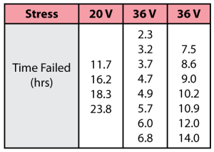
Consider the following times-to-failure data at two different stress levels.
The data set was analyzed jointly in a life-stress data folio using the IPL-Weibull model, with a complete MLE solution over the entire data set. The analysis yields:
IPL-Lognormal
The pdf for the Inverse Power Law relationship and the lognormal distribution is given next.
The pdf of the lognormal distribution is given by:
where:
and:
= times-to-failure.
= mean of the natural logarithms of the times-to-failure.
= standard deviation of the natural logarithms of the times-to-failure.
The median of the lognormal distribution is given by:
The IPL-lognormal model pdf can be obtained first by setting
in the lognormal
pdf. Therefore:
or:
Thus:
So the IPL-lognormal model pdf is:
IPL-Lognormal Statistical Properties Summary
The Mean
The mean life of the IPL-lognormal model (mean of the times-to-failure),
, is given by:
The mean of the natural logarithms of the times-to-failure,
, in terms of
and
is given by:
The Standard Deviation
The standard deviation of the IPL-lognormal model (standard deviation of the times-to-failure),
, is given by:
The standard deviation of the natural logarithms of the times-to-failure,
, in terms of
and
is given by:
The Mode
The mode of the IPL-lognormal model is given by:
IPL-Lognormal Reliability
The reliability for a mission of time T, starting at age 0, for the IPL-lognormal model is determined by:
or:
Reliable Life
The reliable life, or the mission duration for a desired reliability goal,
is estimated by first solving the reliability equation with respect to time, as follows:
where:
and:
Since the reliable life,
, is given by:
Lognormal Failure Rate
The lognormal failure rate is given by:
Parameter Estimation
Maximum Likelihood Estimation Method
The complete IPL-lognormal log-likelihood function is:
where:
and:
is the number of groups of exact times-to-failure data points.
is the number of times-to-failure data points in the
time-to-failure data group.
is the standard deviation of the natural logarithm of the times-to-failure (unknown, the first of three parameters to be estimated).
is the IPL parameter (unknown, the second of three parameters to be estimated).
is the second IPL parameter (unknown, the third of three parameters to be estimated).
is the stress level of the
group.
is the exact failure time of the
group.
is the number of groups of suspension data points.
is the number of suspensions in the
group of suspension data points.
is the running time of the
suspension data group.
is the number of interval data groups.
is the number of intervals in the
group of data intervals.
is the beginning of the
interval.
is the ending of the
interval.
The solution (parameter estimates) will be found by solving for
,
,
so that
,
and
:
and:
IPL and the Coffin-Manson Relationship
In accelerated life testing analysis, thermal cycling is commonly treated as a low-cycle fatigue problem, using the inverse power law relationship. Coffin and Manson suggested that the number of cycles-to-failure of a metal subjected to thermal cycling is given by Nelson [28]:
where:
is the number of cycles to failure.
is a constant, characteristic of the metal.
is another constant, also characteristic of the metal.
is the range of the thermal cycle.
This relationship is basically the inverse power law relationship, where the stress
is substituted by the range
. This is an attempt to simplify the analysis of a time-varying stress test by using a constant stress model. It is a very commonly used methodology for thermal cycling and mechanical fatigue tests. However, by performing such a simplification, the following assumptions and shortcomings are inevitable. First, the acceleration effects due to the stress rate of change are ignored. In other words, it is assumed that the failures are accelerated by the stress difference and not by how rapidly this difference occurs. Secondly, the acceleration effects due to stress relaxation and creep are ignored.
Example
In this example the use of the Coffin-Manson relationship will be illustrated. This is a very simple example which can be repeated at any time. The reader is encouraged to perform this test.
Product: ACME Paper Clip Model 4456
Reliability Target: 99% at a 90% confidence after 30 cycles of 45°
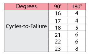
After consulting with our paper-clip engineers, the acceleration stress was determined to be the angle to which the clips are bent. Two bend stresses of 90° and 180° were used. A sample of six paper clips was tested to failure at both 90° and 180° bends with the following data obtained.
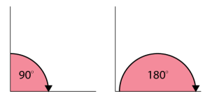
The test was performed as shown in the next figures (a side-view of the paper-clip is shown).
Using the IPL-lognormal model, determine whether the reliability target was met.
Solution
By using the IPL relationship to analyze the data, we are actually using a constant stress model to analyze a cycling process. Caution must be exercised when performing the test. The rate of change in the angle must be constant and equal for both the 90° and 180° bends and constant and equal to the rate of change in the angle for the use life of 45° bend. Rate effects are influencing the life of the paper clip. By keeping the rate constant and equal at all stress levels, we can then eliminate these rate effects from our analysis. Otherwise the analysis will not be valid.
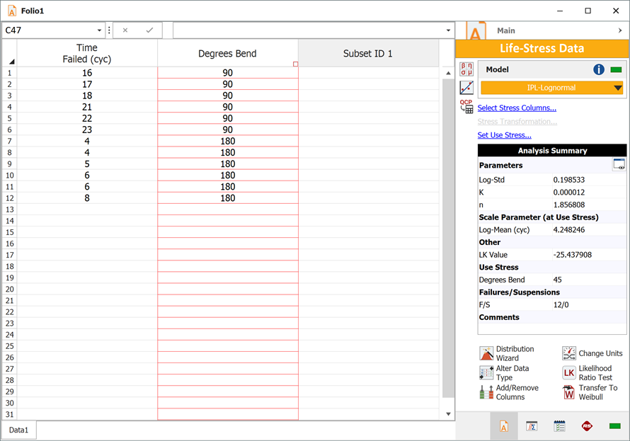
The data were entered and analyzed using ReliaSoft's Weibull++.
The parameters of the IPL-lognormal model were estimated to be:
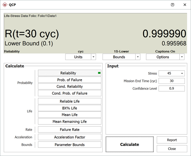
Using the QCP, the 90% lower 1-sided confidence bound on reliability after 30 cycles for a 45° bend was estimated to be
, as shown below.
This meets the target reliability of 99%.
IPL Confidence Bounds
Approximate Confidence Bounds on IPL-Exponential
Confidence Bounds on the Mean Life
From the inverse power law relationship the mean life for the exponential distribution is given by setting
. The upper
and lower
bounds on the mean life (ML estimate of the mean life) are estimated by:
where is defined by:
If is the confidence level, then
for the two-sided bounds, and
for the one-sided bounds. The variance of
is given by:
or:
The variances and covariance of and
are estimated from the Fisher matrix (evaluated at
as follows:
Confidence Bounds on Reliability
The bounds on reliability at a given time,
, are estimated by:
Confidence Bounds on Time
The bounds on time (ML estimate of time) for a given reliability are estimated by first solving the reliability function with respect to time:
The corresponding confidence bounds are estimated from:
Approximate Confidence Bounds on IPL-Weibull
Bounds on the Parameters
Using the same approach as previously discussed (
and
positive parameters):
and:
The variances and covariances of and
are estimated from the local Fisher matrix (evaluated at
as follows:
Confidence Bounds on Reliability
The reliability function (ML estimate) for the IPL-Weibull model is given by:
or:
Setting:
or:
The reliability function now becomes:
The next step is to find the upper and lower bounds on
:
where:
or:
The upper and lower bounds on reliability are:
Confidence Bounds on Time
The bounds on time for a given reliability (ML estimate of time) are estimated by first solving the reliability function with respect to time:
or:
where The upper and lower bounds on
are estimated from:
where:
or:
The upper and lower bounds on time are then found by:
Approximate Confidence Bounds on IPL-Lognormal
Bounds on the Parameters
Since the standard deviation, , and
are positive parameters, then
and
are treated as normally distributed, and the bounds are estimated from:
and:
The lower and upper bounds on , are estimated from:
The variances and covariances of and
are estimated from the local Fisher matrix (evaluated at
,
as follows:
where:
Bounds on Reliability
The reliability of the lognormal distribution is:
Let then
For ,
, and for
The above equation then becomes:
The bounds on are estimated from:
where:
-
.
or:
The upper and lower bounds on reliability are:
Confidence Bounds on Time
The bounds around time, for a given lognormal percentile (unreliability), are estimated by first solving the reliability equation with respect to time, as follows:
where:
and:
The next step is to calculate the variance of
or:
The upper and lower bounds are then found by:
Solving for and
yields:








![{\displaystyle {\begin{aligned}\ln[R({{t}_{R}},V)]=-K{{V}^{n}}{{t}_{R}}\end{aligned}}\,\!}](https://en.wikipedia.org/api/rest_v1/media/math/render/svg/b6a684b9892c7b5693c5a09cd0473e85c96da306)
![{\displaystyle {{t}_{R}}=-{\frac {1}{K{{V}^{n}}}}\ln[R({{t}_{R}},V)]\,\!}](https://en.wikipedia.org/api/rest_v1/media/math/render/svg/ac75ee9d683b4896d4306aa8b802d9e330b263d1)
![{\displaystyle {\begin{aligned}&\ln(L)=\Lambda ={\underset {i=1}{\overset {{F}_{e}}{\mathop {\sum } }}}\,{{N}_{i}}\ln \left[KV_{i}^{n}{{e}^{-KV_{i}^{n}{{T}_{i}}}}\right]-{\underset {i=1}{\overset {S}{\mathop {\sum } }}}\,N_{i}^{\prime }KV_{i}^{n}T_{i}^{\prime }+{\overset {FI}{\mathop {{\underset {i=1}{\mathop {{\underset {}{\overset {}{\mathop {\sum } }}}\,} }}\,} }}\,N_{i}^{\prime \prime }\ln[R_{Li}^{\prime \prime }-R_{Ri}^{\prime \prime }]\end{aligned}}\,\!}](https://en.wikipedia.org/api/rest_v1/media/math/render/svg/a1681b10b5eba828f580e94a22413d56fda30452)


![{\displaystyle R((t|T),V)={\frac {R(T+t,V)}{R(T,V)}}={\frac {{e}^{-{{\left[K{{V}^{n}}\left(T+t\right)\right]}^{\beta }}}}{{e}^{-{{\left(K{{V}^{n}}T\right)}^{\beta }}}}}\,\!}](https://en.wikipedia.org/api/rest_v1/media/math/render/svg/c7c20a7ebe6812caf885ba42179555e4e6b1de48)
![{\displaystyle R((t|T),V)={{e}^{-\left[{{\left(K{{V}^{n}}\left(T+t\right)\right)}^{\beta }}-{{\left(K{{V}^{n}}T\right)}^{\beta }}\right]}}\,\!}](https://en.wikipedia.org/api/rest_v1/media/math/render/svg/f7bd5f1a4f9d452b37eee98208950d7531b1d7c0)

![{\displaystyle {{T}_{R}}={\frac {1}{K{{V}^{n}}}}{{\left\{-\ln \left[R\left({{T}_{R}},V\right)\right]\right\}}^{\tfrac {1}{\beta }}}\,\!}](https://en.wikipedia.org/api/rest_v1/media/math/render/svg/1c4b0551c0ba09964c968173f8e63ce360f7cf49)


![{\displaystyle {\begin{aligned}\Lambda ={\underset {i=1}{\overset {{F}_{e}}{\mathop {\sum } }}}\,{{N}_{i}}\ln \left[\beta KV_{i}^{n}{{\left(KV_{i}^{n}{{T}_{i}}\right)}^{\beta -1}}{{e}^{-{{\left(KV_{i}^{n}{{T}_{i}}\right)}^{\beta }}}}\right]-{\underset {i=1}{\overset {S}{\mathop {\sum } }}}\,N_{i}^{\prime }{{\left(KV_{i}^{n}T_{i}^{\prime }\right)}^{\beta }}+{\overset {FI}{\mathop {{\underset {i=1}{\mathop {{\underset {}{\overset {}{\mathop {\sum } }}}\,} }}\,} }}\,N_{i}^{\prime \prime }\ln[R_{Li}^{\prime \prime }-R_{Ri}^{\prime \prime }]\end{aligned}}\,\!}](https://en.wikipedia.org/api/rest_v1/media/math/render/svg/dce7e852c5dffbdeb13a94cb12c0a71f193e6cf4)


![{\displaystyle {\begin{aligned}{\frac {\partial \Lambda }{\partial \beta }}=\ &{\frac {1}{\beta }}{\underset {i=1}{\overset {{F}_{e}}{\mathop {\sum } }}}\,{{N}_{i}}+{\underset {i=1}{\overset {{F}_{e}}{\mathop {\sum } }}}\,{{N}_{i}}\ln \left(KV_{i}^{n}{{T}_{i}}\right)-{\underset {i=1}{\overset {{F}_{e}}{\mathop {\sum } }}}\,{{N}_{i}}{{\left(KV_{i}^{n}{{T}_{i}}\right)}^{\beta }}\ln \left(KV_{i}^{n}{{T}_{i}}\right)-{\underset {i=1}{\overset {S}{\mathop {\sum } }}}\,N_{i}^{\prime }{{\left(\,KV_{i}^{n}T_{i}^{\prime }\right)}^{\beta }}\ln \left(KV_{i}^{n}T_{i}^{\prime }\right)\\&{\overset {FI}{\mathop {{\underset {i=1}{\mathop {-{\underset {}{\overset {}{\mathop {\sum } }}}\,} }}\,} }}\,N_{i}^{\prime \prime }{\frac {{{\left(KV_{i}^{n}\right)}^{\beta }}\left[R_{Li}^{\prime \prime }T_{Li}^{\prime \prime \beta }\left(\ln(KV_{i}^{n}T_{Li}^{\prime \prime })\right)-R_{Ri}^{\prime \prime }T_{Ri}^{\prime \prime \beta }\left(\ln(KV_{i}^{n}T_{Ri}^{\prime \prime })\right)\right]}{R_{Li}^{\prime \prime }-R_{Ri}^{\prime \prime }}}\\{\frac {\partial \Lambda }{\partial K}}=\ &{\frac {\beta }{K}}{\underset {i=1}{\overset {{F}_{e}}{\mathop {\sum } }}}\,{{N}_{i}}-{\frac {\beta }{K}}{\underset {i=1}{\overset {{F}_{e}}{\mathop {\sum } }}}\,{{N}_{i}}{{\left(KV_{i}^{n}{{T}_{i}}\right)}^{\beta }}-{\frac {\beta }{K}}{\underset {i=1}{\overset {S}{\mathop {\sum } }}}\,N_{i}^{\prime }{{\left(KV_{i}^{n}T_{i}^{\prime }\right)}^{\beta }}{\overset {}{\mathop {-\beta {\underset {i=1}{\mathop {{\overset {FI}{\mathop {{\underset {}{\overset {}{\mathop {\sum } }}}\,} }}\,} }}\,} }}\,N_{i}^{\prime \prime }{\frac {{{K}^{\beta -1}}V_{i}^{n\beta }\left[T_{Li}^{\prime \prime \beta }R_{Li}^{\prime \prime }-T_{Ri}^{\prime \prime \beta }R_{Ri}^{\prime \prime }\right]}{R_{Li}^{\prime \prime }-R_{Ri}^{\prime \prime }}}\\{\frac {\partial \Lambda }{\partial n}}=\ &\beta {\underset {i=1}{\overset {{F}_{e}}{\mathop {\sum } }}}\,{{N}_{i}}\ln({{V}_{i}})-\beta {\underset {i=1}{\overset {{F}_{e}}{\mathop {\sum } }}}\,{{N}_{i}}\ln({{V}_{i}}){{\left(KV_{i}^{n}{{T}_{i}}\right)}^{\beta }}-\beta {\underset {i=1}{\overset {S}{\mathop {\sum } }}}\,N_{i}^{\prime }\ln({{V}_{i}}){{\left(KV_{i}^{n}{{T}_{i}}\right)}^{\beta }}{\overset {FI}{\mathop {{\underset {i=1}{\mathop {-{\underset {}{\overset {}{\mathop {\sum } }}}\,} }}\,} }}\,N_{i}^{\prime \prime }{\frac {n{{K}^{\beta }}V_{i}^{\beta (n-1)}\left[T_{Li}^{\prime \prime \beta }R_{Li}^{\prime \prime }-T_{Ri}^{\prime \prime \beta }R_{Ri}^{\prime \prime }\right]}{R_{Li}^{\prime \prime }-R_{Ri}^{\prime \prime }}}\end{aligned}}\,\!}](https://en.wikipedia.org/api/rest_v1/media/math/render/svg/731b5972d422fef8044a2e60ec8bf2cd0fcdf597)


![{\displaystyle z={{\Phi }^{-1}}\left[F\left(T_{R}^{\prime },\,V\right)\right]\,\!}](https://en.wikipedia.org/api/rest_v1/media/math/render/svg/60a870e2d31d729b5f94bbe92225b324fef9aa1a)


![{\displaystyle {\begin{aligned}\ln(L)=&\Lambda ={\underset {i=1}{\overset {{F}_{e}}{\mathop {\sum } }}}\,{{N}_{i}}\ln \left[{\frac {1}{{{\sigma }_{{T}'}}{{T}_{i}}}}\varphi \left({\frac {\ln \left({{T}_{i}}\right)+\ln(K)+n\ln({{V}_{i}})}{{\sigma }_{{T}'}}}\right)\right]{\text{ }}+{\underset {i=1}{\overset {S}{\mathop {\sum } }}}\,N_{i}^{\prime }\ln \left[1-\Phi \left({\frac {\ln \left(T_{i}^{\prime }\right)+\ln(K)+n\ln({{V}_{i}})}{{\sigma }_{{T}'}}}\right)\right]+{\overset {FI}{\mathop {{\underset {i=1}{\mathop {{\underset {}{\overset {}{\mathop {\sum } }}}\,} }}\,} }}\,N_{i}^{\prime \prime }\ln[\Phi (z_{Ri}^{\prime \prime })-\Phi (z_{Li}^{\prime \prime })]\end{aligned}}\,\!}](https://en.wikipedia.org/api/rest_v1/media/math/render/svg/ce8d2e6405feb460dcf875bbee87e83ebf0f08fe)


![{\displaystyle {\begin{aligned}{\frac {\partial \Lambda }{\partial K}}=&-{\frac {1}{K\cdot \sigma _{{T}'}^{2}}}{\underset {i=1}{\overset {{F}_{e}}{\mathop {\sum } }}}\,{{N}_{i}}(\ln({{T}_{i}})+\ln(K)+n\ln({{V}_{i}}))\ -{\frac {1}{K\cdot {{\sigma }_{{T}'}}}}{\underset {i=1}{\overset {S}{\mathop {\sum } }}}\,N_{i}^{\prime }{\frac {\varphi \left({\tfrac {\ln \left(T_{i}^{\prime }\right)+\ln(K)+n\ln({{V}_{i}})}{{\sigma }_{{T}'}}}\right)}{1-\Phi \left({\tfrac {\ln \left(T_{i}^{\prime }\right)+\ln(K)+n\ln({{V}_{i}})}{{\sigma }_{{T}'}}}\right)}}{\overset {FI}{\mathop {+{\underset {i=1}{\mathop {{\underset {}{\overset {}{\mathop {\sum } }}}\,} }}\,} }}\,N_{i}^{\prime \prime }{\frac {\phi (z_{Ri}^{\prime \prime })-\phi (z_{Li}^{\prime \prime })}{K\sigma _{T}^{\prime }(\Phi (z_{Ri}^{\prime \prime })-\Phi (z_{Li}^{\prime \prime }))}}\\{\frac {\partial \Lambda }{\partial n}}=&-{\frac {1}{\sigma _{{T}'}^{2}}}{\underset {i=1}{\overset {{F}_{e}}{\mathop {\sum } }}}\,{{N}_{i}}\ln({{V}_{i}})\left[\ln({{T}_{i}})+\ln(K)+n\ln({{V}_{i}})\right]-{\frac {1}{{\sigma }_{{T}'}}}{\underset {i=1}{\overset {S}{\mathop {\sum } }}}\,N_{i}^{\prime }\ln({{V}_{i}}){\frac {\varphi \left({\tfrac {\ln \left(T_{i}^{\prime }\right)+\ln(K)+n\ln({{V}_{i}})}{{\sigma }_{{T}'}}}\right)}{1-\Phi \left({\tfrac {\ln \left(T_{i}^{\prime }\right)+\ln(K)+n\ln({{V}_{i}})}{{\sigma }_{{T}'}}}\right)}}+{\overset {FI}{\mathop {{\underset {i=1}{\mathop {{\underset {}{\overset {}{\mathop {\sum } }}}\,} }}\,} }}\,N_{i}^{\prime \prime }{\frac {\ln {{V}_{i}}\left(\phi (z_{Ri}^{\prime \prime })-\phi (z_{Li}^{\prime \prime })\right)}{\sigma _{T}^{\prime }(\Phi (z_{Ri}^{\prime \prime })-\Phi (z_{Li}^{\prime \prime }))}}\\{\frac {\partial \Lambda }{\partial {{\sigma }_{{T}'}}}}=&{\underset {i=1}{\overset {{F}_{e}}{\mathop {\sum } }}}\,{{N}_{i}}\left({\frac {{\left(\ln({{T}_{i}})+\ln(K)+n\ln({{V}_{i}})\right)}^{2}}{\sigma _{{T}'}^{3}}}-{\frac {1}{{\sigma }_{{T}'}}}\right)\ +{\frac {1}{{\sigma }_{{T}'}}}{\underset {i=1}{\overset {S}{\mathop {\sum } }}}\,N_{i}^{\prime }{\frac {\left({\tfrac {\ln \left(T_{i}^{\prime }\right)+\ln(K)+n\ln({{V}_{i}})}{{\sigma }_{{T}'}}}\right)\,\varphi \left({\tfrac {\ln \left(T_{i}^{\prime }\right)+\ln(K)+n\ln({{V}_{i}})}{{\sigma }_{{T}'}}}\right)}{1-\Phi \left({\tfrac {\ln \left(T_{i}^{\prime }\right)+\ln(K)+n\ln({{V}_{i}})}{{\sigma }_{{T}'}}}\right)}}{\overset {FI}{\mathop {{\underset {i=1}{\mathop {-{\underset {}{\overset {}{\mathop {\sum } }}}\,} }}\,} }}\,N_{i}^{\prime \prime }{\frac {z_{Ri}^{\prime \prime }\phi (z_{Ri}^{\prime \prime })-z_{Li}^{\prime \prime }\phi (z_{Li}^{\prime \prime })}{\sigma _{T}^{\prime }(\Phi (z_{Ri}^{\prime \prime })-\Phi (z_{Li}^{\prime \prime }))}}\end{aligned}}\,\!}](https://en.wikipedia.org/api/rest_v1/media/math/render/svg/4b84925e64b1769cae0867d7ed57341dc330bf0f)






![{\displaystyle Var({\widehat {m}})={\frac {1}{{{\widehat {K}}^{2}}{{V}^{2{\widehat {n}}}}}}\left[{\frac {1}{{\widehat {K}}^{2}}}Var({\widehat {K}})+{{\left[\ln(V)\right]}^{2}}Var({\widehat {n}})+{\frac {2\ln(V)}{\widehat {K}}}Cov({\widehat {K}},{\widehat {n}})\right]\,\!}](https://en.wikipedia.org/api/rest_v1/media/math/render/svg/aae3af85b5581f552cd0a66b7dcc0a4e3b25e3c2)

![{\displaystyle \left[{\begin{matrix}Var({\widehat {K}})&Cov({\widehat {K}},{\widehat {n}})\\Cov({\widehat {n}},{\widehat {K}})&Var({\widehat {n}})\\\end{matrix}}\right]={{\left[{\begin{matrix}-{\tfrac {{{\partial }^{2}}\Lambda }{\partial {{K}^{2}}}}&-{\tfrac {{{\partial }^{2}}\Lambda }{\partial K\partial n}}\\-{\tfrac {{{\partial }^{2}}\Lambda }{\partial n\partial K}}&-{\tfrac {{{\partial }^{2}}\Lambda }{\partial {{n}^{2}}}}\\\end{matrix}}\right]}^{-1}}\,\!}](https://en.wikipedia.org/api/rest_v1/media/math/render/svg/f0a0a38de08e40f5938e88084111f4fe444926ba)


![{\displaystyle \left[{\begin{matrix}Var({\widehat {\beta }})&Cov({\widehat {\beta }},{\widehat {K}})&Cov({\widehat {\beta }},{\widehat {n}})\\Cov({\widehat {K}},{\widehat {\beta }})&Var({\widehat {K}})&Cov({\widehat {K}},{\widehat {n}})\\Cov({\widehat {n}},{\widehat {\beta }})&Cov({\widehat {n}},{\widehat {K}})&Var({\widehat {n}})\\\end{matrix}}\right]={{\left[{\begin{matrix}-{\tfrac {{{\partial }^{2}}\Lambda }{\partial {{\beta }^{2}}}}&-{\tfrac {{{\partial }^{2}}\Lambda }{\partial \beta \partial K}}&-{\tfrac {{{\partial }^{2}}\Lambda }{\partial \beta \partial n}}\\-{\tfrac {{{\partial }^{2}}\Lambda }{\partial K\partial \beta }}&-{\tfrac {{{\partial }^{2}}\Lambda }{\partial {{K}^{2}}}}&-{\tfrac {{{\partial }^{2}}\Lambda }{\partial K\partial n}}\\-{\tfrac {{{\partial }^{2}}\Lambda }{\partial n\partial \beta }}&-{\tfrac {{{\partial }^{2}}\Lambda }{\partial n\partial A}}&-{\tfrac {{{\partial }^{2}}\Lambda }{\partial {{n}^{2}}}}\\\end{matrix}}\right]}^{-1}}\,\!}](https://en.wikipedia.org/api/rest_v1/media/math/render/svg/1b801e6da8faa2c79766f521238b62347d927730)

![{\displaystyle {\widehat {R}}(T,V)={{e}^{-{{e}^{\ln \left[{{\left({\widehat {K}}{{V}^{\widehat {n}}}T\right)}^{\widehat {\beta }}}\right]}}}}\,\!}](https://en.wikipedia.org/api/rest_v1/media/math/render/svg/a28522e9afa7f72e8f1b87f39356319d8aca2d58)
![{\displaystyle {\widehat {u}}=\ln \left[\left({\widehat {K}}V{\widehat {^{n}}}T\right){\widehat {^{\beta }}}\right]\,\!}](https://en.wikipedia.org/api/rest_v1/media/math/render/svg/37d780eb5c1261a354e9d2c10c17e8f38e3fd11b)
![{\displaystyle {\widehat {u}}={\widehat {\beta }}\left[\ln(T)+\ln({\widehat {K}})+{\widehat {n}}\ln(V)\right]\,\!}](https://en.wikipedia.org/api/rest_v1/media/math/render/svg/beef7ac5467085bc41b5ea6304722e8fb508452e)


![{\displaystyle {\begin{aligned}&Var({\widehat {u}})=&{{\left({\frac {\widehat {u}}{\widehat {\beta }}}\right)}^{2}}Var({\widehat {\beta }})+{{\left({\frac {\widehat {\beta }}{\widehat {K}}}\right)}^{2}}Var({\widehat {K}})+{{\widehat {\beta }}^{2}}{{\left[\ln(V)\right]}^{2}}Var({\widehat {n}})+{\frac {2{\widehat {u}}}{\widehat {K}}}Cov({\widehat {\beta }},{\widehat {K}})+2{\widehat {u}}\ln(V)Cov({\widehat {\beta }},{\widehat {n}})+{\frac {2{{\widehat {\beta }}^{2}}\ln(V)}{\widehat {K}}}Cov({\widehat {K}},{\widehat {n}})\end{aligned}}\,\!}](https://en.wikipedia.org/api/rest_v1/media/math/render/svg/fa1a549dc4bee78a43a062261b429b9d3e783fb8)

![{\displaystyle {\begin{aligned}\ln(R)&=\ -{{\left({\widehat {K}}{{V}^{\widehat {n}}}{\widehat {T}}\right)}^{\widehat {\beta }}}\\\ln(-\ln(R))&=\ {\widehat {\beta }}\left[\ln({\widehat {T}})+\ln({\widehat {K}})+{\widehat {n}}\ln(V)\right]\end{aligned}}\,\!}](https://en.wikipedia.org/api/rest_v1/media/math/render/svg/4839637f1f612367932c125ae6ccf0d4a4f2a7a6)


![{\displaystyle {\begin{aligned}Var({\widehat {u}})=&{\frac {1}{{\widehat {\beta }}^{4}}}{{\left[\ln(-\ln(R))\right]}^{2}}Var({\widehat {\beta }})+{\frac {1}{{\widehat {K}}^{2}}}Var({\widehat {K}})+{{\left[\ln(V)\right]}^{2}}Var({\widehat {n}})+{\frac {2\ln(-\ln(R))}{{{\widehat {\beta }}^{2}}{\widehat {K}}}}Cov({\widehat {\beta }},{\widehat {K}})\\&+{\frac {2\ln(-\ln(R))}{{\widehat {\beta }}^{2}}}\ln(V)Cov({\widehat {\beta }},{\widehat {n}})+{\frac {2\ln(V)}{\widehat {K}}}Cov({\widehat {K}},{\widehat {n}})\end{aligned}}\,\!}](https://en.wikipedia.org/api/rest_v1/media/math/render/svg/2bf00c299787abedddbf9a5c56a876638647ac18)


![{\displaystyle \left[{\begin{matrix}Var({{\widehat {\sigma }}_{{T}'}})&Cov({\widehat {K}},{{\widehat {\sigma }}_{{T}'}})&Cov({\widehat {n}},{{\widehat {\sigma }}_{{T}'}})\\Cov({{\widehat {\sigma }}_{{T}'}},{\widehat {K}})&Var({\widehat {K}})&Cov({\widehat {K}},{\widehat {n}})\\Cov({{\widehat {\sigma }}_{{T}'}},{\widehat {n}})&Cov({\widehat {n}},{\widehat {K}})&Var\left({\widehat {n}}\right)\\\end{matrix}}\right]={{\left[F\right]}^{-1}}\,\!}](https://en.wikipedia.org/api/rest_v1/media/math/render/svg/169046154e60581f2b26aa548c8e0e9e58db0d82)
![{\displaystyle F=\left[{\begin{matrix}-{\tfrac {{{\partial }^{2}}\Lambda }{\partial \sigma _{{T}'}^{2}}}&-{\tfrac {{{\partial }^{2}}\Lambda }{\partial {{\sigma }_{{T}'}}\partial K}}&-{\tfrac {{{\partial }^{2}}\Lambda }{\partial {{\sigma }_{{T}'}}\partial n}}\\-{\tfrac {{{\partial }^{2}}\Lambda }{\partial K\partial {{\sigma }_{{T}'}}}}&-{\tfrac {{{\partial }^{2}}\Lambda }{\partial {{K}^{2}}}}&-{\tfrac {{{\partial }^{2}}\Lambda }{\partial K\partial n}}\\-{\tfrac {{{\partial }^{2}}\Lambda }{\partial n\partial {{\sigma }_{{T}'}}}}&-{\tfrac {{{\partial }^{2}}\Lambda }{\partial n\partial K}}&-{\tfrac {{{\partial }^{2}}\Lambda }{\partial {{n}^{2}}}}\\\end{matrix}}\right]\,\!}](https://en.wikipedia.org/api/rest_v1/media/math/render/svg/8ae3dbda1a912886366819796ee5d3aba7b2f2e8)


![{\displaystyle {\begin{aligned}&Var({\widehat {z}})=&{\frac {1}{{\widehat {\sigma }}_{{T}'}^{2}}}[{\frac {1}{{K}^{2}}}Var({\widehat {K}})+\ln {{(V)}^{2}}Var({\widehat {n}})+{{\widehat {z}}^{2}}Var({{\widehat {\sigma }}_{{T}'}})+{\frac {2\ln(V)}{K}}Cov\left({\widehat {K}},{\widehat {n}}\right)-{\frac {2{\widehat {z}}}{K}}Cov\left({\widehat {K}},{{\widehat {\sigma }}_{{T}'}}\right)-2{\widehat {z}}\ln(V)Cov\left({\widehat {n}},{{\widehat {\sigma }}_{{T}'}}\right)]\end{aligned}}\,\!}](https://en.wikipedia.org/api/rest_v1/media/math/render/svg/dcf6a0d817dcfab042e33fad800ace377d6d5948)


![{\displaystyle {\begin{aligned}&{T}'(V;{\widehat {K}},{\widehat {n}},{{\widehat {\sigma }}_{{T}'}})=\ \ln(T)\\\\&z=\ {{\Phi }^{-1}}\left[F({T}')\right]\end{aligned}}\,\!}](https://en.wikipedia.org/api/rest_v1/media/math/render/svg/4fddcb8ccb39086d4ec98511adcb49738a0f76d8)


