Eyring Relationship
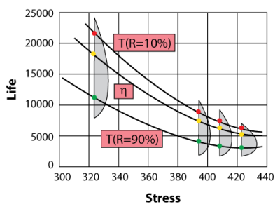
The Eyring relationship was formulated from quantum mechanics principles, as discussed in Glasstone et al. [9], and is most often used when thermal stress (temperature) is the acceleration variable. However, the Eyring relationship is also often used for stress variables other than temperature, such as humidity. The relationship is given by:
where:
represents a quantifiable life measure, such as mean life, characteristic life, median life,
life, etc.
represents the stress level (temperature values are in absolute units: kelvin or degrees Rankine).
is one of the model parameters to be determined.
is another model parameter to be determined.
The Eyring relationship is similar to the Arrhenius relationship. This similarity is more apparent if it is rewritten in the following way:
or:
The Arrhenius relationship is given by:
Comparing the above equation to the Arrhenius relationship, it can be seen that the only difference between the two relationships is the
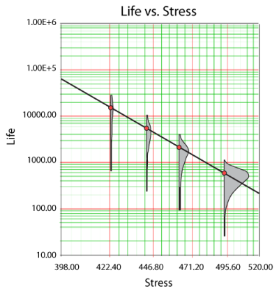
term above. In general, both relationships yield very similar results. Like the Arrhenius, the Eyring relationship is plotted on a log-reciprocal paper.
Acceleration Factor
For the Eyring model the acceleration factor is given by:
Eyring-Exponential
The pdf of the 1-parameter exponential distribution is given by:
It can be easily shown that the mean life for the 1-parameter exponential distribution (presented in detail here) is given by:
thus:
The Eyring-exponential model pdf can then be obtained by setting
:
and substituting for in the exponential
pdf equation:
Eyring-Exponential Statistical Properties Summary
Mean or MTTF
The mean, or Mean Time To Failure (MTTF) for the Eyring-exponential is given by:
Median
The median,
for the Eyring-exponential model is given by:
Mode
The mode,
for the Eyring-exponential model is
Standard Deviation
The standard deviation, , for the Eyring-exponential model is given by:
Eyring-Exponential Reliability Function
The Eyring-exponential reliability function is given by:
This function is the complement of the Eyring-exponential cumulative distribution function or:
and:
Conditional Reliability
The conditional reliability function for the Eyring-exponential model is given by:
Reliable Life
For the Eyring-exponential model, the reliable life, or the mission duration for a desired reliability goal,
is given by:
or:
Parameter Estimation
Maximum Likelihood Estimation Method
The complete exponential log-likelihood function of the Eyring model is composed of two summation portions:
- where:
and:
is the number of groups of exact times-to-failure data points.
is the number of times-to-failure in the
time-to-failure data group.
is the stress level of the
group.
is the Eyring parameter (unknown, the first of two parameters to be estimated).
is the second Eyring parameter (unknown, the second of two parameters to be estimated).
is the exact failure time of the
group.
is the number of groups of suspension data points.
is the number of suspensions in the
group of suspension data points.
is the running time of the
suspension data group.
is the number of interval data groups.
is the number of intervals in the
group of data intervals.
is the beginning of the
interval.
is the ending of the
interval.
The solution (parameter estimates) will be found by solving for the parameters
and
so that
and
where:
Eyring-Weibull
The pdf for 2-parameter Weibull distribution is given by:
The scale parameter (or characteristic life) of the Weibull distribution is
. The Eyring-Weibull model
pdf can then be obtained by setting
:
or:
Substituting for into the Weibull
pdf yields:
Eyring-Weibull Statistical Properties Summary
Mean or MTTF
The mean, , or Mean Time To Failure (MTTF) for the Eyring-Weibull model is given by:
where is the gamma function evaluated at the value of
.
Median
The median,
for the Eyring-Weibull model is given by:
Mode
The mode,
for the Eyring-Weibull model is given by:
Standard Deviation
The standard deviation,
for the Eyring-Weibull model is given by:
Eyring-Weibull Reliability Function
The Eyring-Weibull reliability function is given by:
Conditional Reliability Function
The Eyring-Weibull conditional reliability function at a specified stress level is given by:
or:
Reliable Life
For the Eyring-Weibull model, the reliable life,
, of a unit for a specified reliability and starting the mission at age zero is given by:
Eyring-Weibull Failure Rate Function
The Eyring-Weibull failure rate function,
, is given by:
Parameter Estimation
Maximum Likelihood Estimation Method
The Eyring-Weibull log-likelihood function is composed of two summation portions:
where:
and:
is the number of groups of exact times-to-failure data points.
is the number of times-to-failure data points in the
time-to-failure data group.
is the Weibull shape parameter (unknown, the first of three parameters to be estimated).
is the Eyring parameter (unknown, the second of three parameters to be estimated).
is the second Eyring parameter (unknown, the third of three parameters to be estimated).
is the stress level of the
group.
is the exact failure time of the
group.
is the number of groups of suspension data points.
is the number of suspensions in the
group of suspension data points.
is the running time of the
suspension data group.
is the number of interval data groups.
is the number of intervals in the
group of data intervals.
is the beginning of the
interval.
is the ending of the
interval.
The solution (parameter estimates) will be found by solving for the parameters
and
so that
and
where:
Eyring-Weibull Example
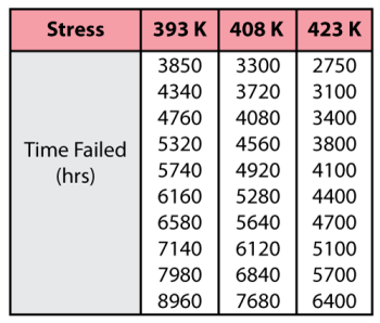
Consider the following times-to-failure data at three different stress levels.
The data set was entered into the life-stress data folio and analyzed using the Eyring-Weibull model, yielding:
Once the parameters of the model are defined, other life measures can be directly obtained using the appropriate equations. For example, the MTTF can be obtained for the use stress level of 323 K by using:
or:
Eyring-Lognormal
The pdf of the lognormal distribution is given by:
where:
and
mean of the natural logarithms of the times-to-failure.
standard deviation of the natural logarithms of the times-to-failure.
The Eyring-lognormal model can be obtained first by setting
:
or:
Thus:
Substituting this into the lognormal pdf yields the Eyring-lognormal model pdf:
Eyring-Lognormal Statistical Properties Summary
The Mean
The mean life of the Eyring-lognormal model (mean of the times-to-failure),
, is given by:
The mean of the natural logarithms of the times-to-failure,
, in terms of
and
is given by:
The Median
The median of the Eyring-lognormal model is given by:
The Standard Deviation
The standard deviation of the Eyring-lognormal model (standard deviation of the times-to-failure),
, is given by:
The standard deviation of the natural logarithms of the times-to-failure,
, in terms of
and
is given by:
The Mode
The mode of the Eyring-lognormal model is given by:
Eyring-Lognormal Reliability Function
The reliability for a mission of time
, starting at age 0, for the Eyring-lognormal model is determined by:
or:
There is no closed form solution for the lognormal reliability function. Solutions can be obtained via the use of standard normal tables. Since the application automatically solves for the reliability we will not discuss manual solution methods.
Reliable Life
For the Eyring-lognormal model, the reliable life, or the mission duration for a desired reliability goal,
is estimated by first solving the reliability equation with respect to time, as follows:
where:
and:
Since the reliable life,
is given by:
Eyring-Lognormal Failure Rate
The Eyring-lognormal failure rate is given by:
Parameter Estimation
Maximum Likelihood Estimation Method
The complete Eyring-lognormal log-likelihood function is composed of two summation portions:
where:
and:
is the number of groups of exact times-to-failure data points.
is the number of times-to-failure data points in the
time-to-failure data group.
is the standard deviation of the natural logarithm of the times-to-failure (unknown, the first of three parameters to be estimated).
is the Eyring parameter (unknown, the second of three parameters to be estimated).
is the second Eyring parameter (unknown, the third of three parameters to be estimated).
is the stress level of the
group.
is the exact failure time of the
group.
is the number of groups of suspension data points.
is the number of suspensions in the
group of suspension data points.
is the running time of the
suspension data group.
is the number of interval data groups.
is the number of intervals in the
group of data intervals.
is the beginning of the
interval.
is the ending of the
interval.
The solution (parameter estimates) will be found by solving for
so that
and
:
and:
Generalized Eyring Relationship
The generalized Eyring relationship is used when temperature and a second non-thermal stress (e.g. voltage) are the accelerated stresses of a test and their interaction is also of interest. This relationship is given by:
where:
is the temperature (in absolute units).
is the non-thermal stress (i.e., voltage, vibration, etc.).
are the parameters to be determined.
The Eyring relationship is a simple case of the generalized Eyring relationship where
and
Note that the generalized Eyring relationship includes the interaction term of
and
as described by the
term. In other words, this model can estimate the effect of changing one of the factors depending on the level of the other factor.
Acceleration Factor
Most models in actual use do not include any interaction terms, therefore, the acceleration factor can be computed by multiplying the acceleration factors obtained by changing each factor while keeping the other factors constant. In the case of the generalized Eyring relationship, the acceleration factor is derived differently.
The acceleration factor for the generalized Eyring relationship is given by:
where:
is the life at use stress level.
is the life at the accelerated stress level.
is the use temperature level.
is the accelerated temperature level.
is the accelerated non-thermal level.
is the use non-thermal level.
Generalized Eyring-Exponential
By setting , the exponential
pdf becomes:
Generalized Eyring-Exponential Reliability Function
The generalized Eyring exponential model reliability function is given by:
Parameter Estimation
Substituting the generalized Eyring model into the lognormal log-likelihood equation yields:
where:
and:
is the number of groups of exact times-to-failure data points.
is the number of times-to-failure data points in the
time-to-failure data group.
are parameters to be estimated.
is the temperature level of the
group.
is the non-thermal stress level of the
group.
is the exact failure time of the
group.
is the number of groups of suspension data points.
is the number of suspensions in the
group of suspension data points.
is the running time of the
suspension data group.
is the number of interval data groups.
is the number of intervals in the
group of data intervals.
is the beginning of the
interval.
is the ending of the
interval.
The solution (parameter estimates) will be found by solving for the parameters
and
so that
and
.
Generalized Eyring-Weibull
By setting to the Weibull
pdf, the generalized Eyring Weibull model is given by:
Generalized Eyring-Weibull Reliability Function
The generalized Eyring Weibull reliability function is given by:
Parameter Estimation
Substituting the generalized Eyring model into the Weibull log-likelihood equation yields:
where:
and:
is the number of groups of exact times-to-failure data points.
is the number of times-to-failure data points in the
time-to-failure data group.
are parameters to be estimated.
is the temperature level of the
group.
is the non-thermal stress level of the
group.
is the exact failure time of the
group.
is the number of groups of suspension data points.
is the number of suspensions in the
group of suspension data points.
is the running time of the
suspension data group.
is the number of interval data groups.
is the number of intervals in the
group of data intervals.
is the beginning of the
interval.
is the ending of the
interval.
The solution (parameter estimates) will be found by solving for the parameters
and
so that
and
.
Generalized Eyring-Lognormal
By setting to the lognormal
pdf, the generalized Erying lognormal model is given by:
where:
Generalized Eyring-Lognormal Reliability Function
The generalized Erying lognormal reliability function is given by:
Parameter Estimation
Substituting the generalized Eyring model into the lognormal log-likelihood equation yields:
where:
and:
is the number of groups of exact times-to-failure data points.
is the number of times-to-failure data points in the
time-to-failure data group.
are parameters to be estimated.
is the temperature level of the
group.
is the non-thermal stress level of the
group.
is the exact failure time of the
group.
is the number of groups of suspension data points.
is the number of suspensions in the
group of suspension data points.
is the running time of the
suspension data group.
is the number of interval data groups.
is the number of intervals in the
group of data intervals.
is the beginning of the
interval.
is the ending of the
interval.
The solution (parameter estimates) will be found by solving for the parameters
and
so that
and
.
Generalized Eyring Example
The following data set represents failure times (in hours) obtained from an electronics epoxy packaging accelerated life test performed to understand the synergy between temperature and humidity and estimate the
life at the use conditions of
and
. The data set is modeled using the lognormal distribution and the generalized Eyring model.
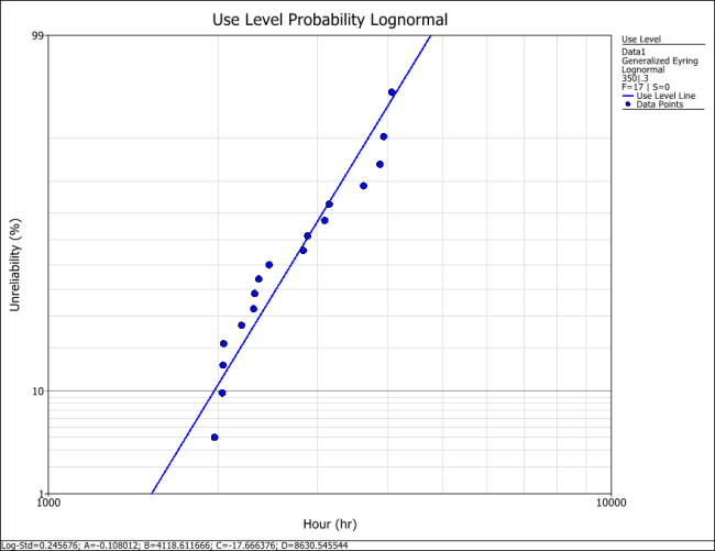
The probability plot at the use conditions is shown next.
The information is estimated to be 1967.2 hours, as shown next.
Eyring Confidence Bounds
Approximate Confidence Bounds for the Eyring-Exponential
Confidence Bounds on Mean Life
The mean life for the Eyring relationship is given by setting
. The upper
and lower
bounds on the mean life (ML estimate of the mean life) are estimated by:
where is defined by:
If is the confidence level, then
for the two-sided bounds, and
for the one-sided bounds. The variance of
is given by:
or:
The variances and covariance of and
are estimated from the local Fisher matrix (evaluated at
,
as follows:
Confidence Bounds on Reliability
The bounds on reliability at a given time,
, are estimated by:
Confidence Bounds on Time
The bounds on time (ML estimate of time) for a given reliability are estimated by first solving the reliability function with respect to time:
The corresponding confidence bounds are estimated from:
Approximate Confidence Bounds for the Eyring-Weibull
Bounds on the Parameters
From the asymptotically normal property of the maximum likelihood estimators, and since
is a positive parameter,
can then be treated as normally distributed. After performing this transformation, the bounds on the parameters are estimated from:
also:
and:
The variances and covariances of and
are estimated from the Fisher matrix (evaluated at
as follows:
Confidence Bounds on Reliability
The reliability function for the Eyring-Weibull model (ML estimate) is given by:
or:
Setting:
or:
The reliability function now becomes:
The next step is to find the upper and lower bounds on
:
where:
or:
The upper and lower bounds on reliability are:
Confidence Bounds on Time
The bounds on time (ML estimate of time) for a given reliability are estimated by first solving the reliability function with respect to time:
or:
where . The upper and lower bounds on
are then estimated from:
where:
or:
The upper and lower bounds on time are then found by:
Approximate Confidence Bounds for the Eyring-Lognormal
Bounds on the Parameters
The lower and upper bounds on and
are estimated from:
and:
Since the standard deviation, is a positive parameter,
is treated as normally distributed, and the bounds are estimated from:
The variances and covariances of and
are estimated from the local Fisher matrix (evaluated at
,
as follows:
where:
Bounds on Reliability
The reliability of the lognormal distribution is given by:
Let then
For ,
, and for
The above equation then becomes:
The bounds on are estimated from:
where:
or:
The upper and lower bounds on reliability are:
Confidence Bounds on Time
The bounds around time for a given lognormal percentile (unreliability) are estimated by first solving the reliability equation with respect to time as follows:
where:
and:
The next step is to calculate the variance of
or:
The upper and lower bounds are then found by:
Solving for and
yields:


![{\displaystyle \ln[R({{t}_{R}},V)]=-{{t}_{R}}\cdot V\cdot {{e}^{\left(A-{\tfrac {B}{V}}\right)}}\,\!}](https://en.wikipedia.org/api/rest_v1/media/math/render/svg/86cd982daf8e0e98c92f33245f2d19a11e7add5c)
![{\displaystyle {{t}_{R}}=-{\frac {1}{V}}{{e}^{-\left(A-{\tfrac {B}{V}}\right)}}\ln[R({{t}_{R}},V)]\,\!}](https://en.wikipedia.org/api/rest_v1/media/math/render/svg/5202449c1764671b627f12553e201e76f38adfb1)
![{\displaystyle {\begin{aligned}&\ln(L)=&\Lambda ={\underset {i=1}{\overset {{F}_{e}}{\mathop {\sum } }}}\,{{N}_{i}}\ln \left[{{V}_{i}}\cdot {{e}^{\left(A-{\tfrac {B}{{V}_{i}}}\right)}}{{e}^{-{{V}_{i}}\cdot {{e}^{\left(A-{\tfrac {B}{{V}_{i}}}\right)}}\cdot {{T}_{i}}}}\right]-{\underset {i=1}{\overset {S}{\mathop {\sum } }}}\,N_{i}^{\prime }\cdot {{V}_{i}}\cdot {{e}^{\left(A-{\tfrac {B}{{V}_{i}}}\right)}}\cdot T_{i}^{\prime }+{\overset {FI}{\mathop {{\underset {i=1}{\mathop {{\underset {}{\overset {}{\mathop {\sum } }}}\,} }}\,} }}\,N_{i}^{\prime \prime }\ln[R_{Li}^{\prime \prime }-R_{Ri}^{\prime \prime }]\end{aligned}}\,\!}](https://en.wikipedia.org/api/rest_v1/media/math/render/svg/bf0bb72ae99e29d0aee6cc5d68e37de248e5337d)


![{\displaystyle {\begin{aligned}&{\frac {\partial \Lambda }{\partial B}}=&{\underset {i=1}{\overset {{F}_{e}}{\mathop {\sum } }}}\,{{N}_{i}}\left[{{e}^{\left(A-{\tfrac {B}{{V}_{i}}}\right)}}{{T}_{i}}-{\frac {1}{{V}_{i}}}\right]+{\underset {i=1}{\overset {S}{\mathop {\sum } }}}\,N_{i}^{\prime }\cdot {{e}^{\left(A-{\tfrac {B}{{V}_{i}}}\right)}}T_{i}^{\prime }{\overset {FI}{\mathop {{\underset {i=1}{\mathop {+{\underset {}{\overset {}{\mathop {\sum } }}}\,} }}\,} }}\,N_{i}^{\prime \prime }{\frac {\left(T_{Li}^{\prime \prime }R_{Li}^{\prime \prime }-T_{Ri}^{\prime \prime }R_{Ri}^{\prime \prime }\right){{e}^{A-{\tfrac {B}{{V}_{i}}}}}}{R_{Li}^{\prime \prime }-R_{Ri}^{\prime \prime }}}\end{aligned}}\,\!}](https://en.wikipedia.org/api/rest_v1/media/math/render/svg/67a3edcc85289716f3911c7f1f3ac53c37572365)


![{\displaystyle R((t|T),V)={{e}^{-\left[{{\left(\left(T+t\right)\cdot V\cdot {{e}^{\left(A-{\tfrac {B}{V}}\right)}}\right)}^{\beta }}-{{\left(V\cdot T\cdot {{e}^{\left(A-{\tfrac {B}{V}}\right)}}\right)}^{\beta }}\right]}}\,\!}](https://en.wikipedia.org/api/rest_v1/media/math/render/svg/dc018563111d619fe22b26ebf04b87b84fcaaf45)

![{\displaystyle {{t}_{R}}={\frac {1}{V}}{{e}^{-\left(A-{\tfrac {B}{V}}\right)}}{{\left\{-\ln \left[R\left({{T}_{R}},V\right)\right]\right\}}^{\tfrac {1}{\beta }}}\,\!}](https://en.wikipedia.org/api/rest_v1/media/math/render/svg/05cec1c3ca57f6c0d1757e2141bf04d54d2f8600)


![{\displaystyle {\begin{aligned}&\ln(L)=&\Lambda ={\underset {i=1}{\overset {{F}_{e}}{\mathop {\sum } }}}\,{{N}_{i}}\ln \left[\beta \cdot {{V}_{i}}\cdot {{e}^{A-{\tfrac {B}{{V}_{i}}}}}{{\left({{T}_{i}}{{V}_{i}}{{e}^{A-{\tfrac {B}{{V}_{i}}}}}\right)}^{\beta -1}}{{e}^{-{{\left({{T}_{i}}{{V}_{i}}{{e}^{A-{\tfrac {B}{{V}_{i}}}}}\right)}^{\beta }}}}\right]-{\underset {i=1}{\overset {S}{\mathop {\sum } }}}\,N_{i}^{\prime }{{\left({{V}_{i}}{{e}^{A-{\tfrac {B}{{V}_{i}}}}}T_{i}^{\prime }\right)}^{\beta }}+{\overset {FI}{\mathop {{\underset {i=1}{\mathop {{\underset {}{\overset {}{\mathop {\sum } }}}\,} }}\,} }}\,N_{i}^{\prime \prime }\ln[R_{Li}^{\prime \prime }-R_{Ri}^{\prime \prime }]\end{aligned}}\,\!}](https://en.wikipedia.org/api/rest_v1/media/math/render/svg/3655749700ee4a47a5b838007d3b5d5d0bd9e5eb)


![{\displaystyle {\begin{aligned}&{\frac {\partial \Lambda }{\partial A}}=&\beta {\underset {i=1}{\overset {{F}_{e}}{\mathop {\sum } }}}\,{{N}_{i}}-\beta {\underset {i=1}{\overset {{F}_{e}}{\mathop {\sum } }}}\,{{N}_{i}}{{\left({{T}_{i}}{{V}_{i}}{{e}^{A-{\tfrac {B}{{V}_{i}}}}}\right)}^{\beta }}-\beta {\underset {i=1}{\overset {S}{\mathop {\sum } }}}\,N_{i}^{\prime }{{\left(T_{i}^{\prime }{{V}_{i}}{{e}^{A-{\tfrac {B}{{V}_{i}}}}}\right)}^{\beta }}{\overset {FI}{\mathop {-{\underset {i=1}{\mathop {{\underset {}{\overset {}{\mathop {\sum } }}}\,} }}\,} }}\,N_{i}^{\prime \prime }{\frac {\beta V_{i}^{\beta }{{e}^{A\beta -{\tfrac {B\beta }{{V}_{i}}}}}\left[{{(T_{Li}^{\prime \prime })}^{\beta }}R_{Li}^{\prime \prime }-{{(T_{Ri}^{\prime \prime })}^{\beta }}R_{Ri}^{\prime \prime }\right]}{R_{Li}^{\prime \prime }-R_{Ri}^{\prime \prime }}}\end{aligned}}\,\!}](https://en.wikipedia.org/api/rest_v1/media/math/render/svg/536b4c45859f67eaf1844a7edcc599cbc393a706)
![{\displaystyle {\begin{aligned}&{\frac {\partial \Lambda }{\partial B}}=&-\beta {\underset {i=1}{\overset {{F}_{e}}{\mathop {\sum } }}}\,{{N}_{i}}{\frac {1}{{V}_{i}}}+\beta {\underset {i=1}{\overset {{F}_{e}}{\mathop {\sum } }}}\,{{N}_{i}}{\frac {1}{{V}_{i}}}{{\left({{T}_{i}}{{V}_{i}}{{e}^{A-{\tfrac {B}{{V}_{i}}}}}\right)}^{\beta }}+\beta {\underset {i=1}{\overset {S}{\mathop {\sum } }}}\,N_{i}^{\prime }{\frac {1}{{V}_{i}}}{{\left(T_{i}^{\prime }{{V}_{i}}{{e}^{A-{\tfrac {B}{{V}_{i}}}}}\right)}^{\beta }}+{\overset {FI}{\mathop {{\underset {i=1}{\mathop {{\underset {}{\overset {}{\mathop {\sum } }}}\,} }}\,} }}\,N_{i}^{\prime \prime }{\frac {\beta V_{i}^{(\beta -1)}{{e}^{A\beta -{\tfrac {B\beta }{{V}_{i}}}}}\left[{{(T_{Li}^{\prime \prime })}^{\beta }}R_{Li}^{\prime \prime }-{{(T_{Ri}^{\prime \prime })}^{\beta }}R_{Ri}^{\prime \prime }\right]}{R_{Li}^{\prime \prime }-R_{Ri}^{\prime \prime }}}\end{aligned}}\,\!}](https://en.wikipedia.org/api/rest_v1/media/math/render/svg/8a4d21e5a7f13a8662e1c44cffc56d9d2d90d355)


![{\displaystyle z={{\Phi }^{-1}}\left[F\left(T_{R}^{\prime },V\right)\right]\,\!}](https://en.wikipedia.org/api/rest_v1/media/math/render/svg/5d8c788033ad77314ac427e047fc6c7bccd5b875)


![{\displaystyle {\begin{aligned}&\ln(L)=&\Lambda ={\underset {i=1}{\overset {{F}_{e}}{\mathop {\sum } }}}\,{{N}_{i}}\ln \left[{\frac {1}{{{\sigma }_{{T}'}}{{T}_{i}}}}\phi \left({\frac {\ln \left({{T}_{i}}\right)+\ln({{V}_{i}})+A-{\tfrac {B}{{V}_{i}}}}{{\sigma }_{{T}'}}}\right)\right]{\text{ }}+{\underset {i=1}{\overset {S}{\mathop {\sum } }}}\,N_{i}^{\prime }\ln \left[1-\Phi \left({\frac {\ln \left(T_{i}^{\prime }\right)+\ln({{V}_{i}})+A-{\tfrac {B}{{V}_{i}}}}{{\sigma }_{{T}'}}}\right)\right]+{\overset {FI}{\mathop {{\underset {i=1}{\mathop {{\underset {}{\overset {}{\mathop {\sum } }}}\,} }}\,} }}\,N_{i}^{\prime \prime }\ln[\Phi (z_{Ri}^{\prime \prime })-\Phi (z_{Li}^{\prime \prime })]\end{aligned}}\,\!}](https://en.wikipedia.org/api/rest_v1/media/math/render/svg/7b42183969372a958ccca9ad72c5f74d823b5adf)


![{\displaystyle {\begin{aligned}&\ln(L)=&\Lambda ={\overset {Fe}{\mathop {{\underset {i=1}{\mathop {{\underset {}{\overset {}{\mathop {\sum } }}}\,} }}\,} }}\,{{N}_{i}}\ln[{\frac {\varphi (z(t))}{\sigma _{T}^{\prime }t}}]{\overset {S}{\mathop {{\underset {i=1}{\mathop {+{\underset {}{\overset {}{\mathop {\sum } }}}\,} }}\,} }}\,N_{i}^{\prime }\ln \left(1-\Phi (z(t_{i}^{\prime }))\right)+{\overset {FI}{\mathop {{\underset {i=1}{\mathop {{\underset {}{\overset {}{\mathop {\sum } }}}\,} }}\,} }}\,N_{i}^{\prime \prime }\ln[\Phi (z_{Ri}^{\prime \prime })-\Phi (z_{Li}^{\prime \prime })]\end{aligned}}\,\!}](https://en.wikipedia.org/api/rest_v1/media/math/render/svg/849c0e9b8c528f12f200ea9927aa14abac9947ec)


![{\displaystyle {\begin{aligned}\ln(L)=\Lambda =&{\overset {Fe}{\mathop {{\underset {i=1}{\mathop {{\underset {}{\overset {}{\mathop {\sum } }}}\,} }}\,} }}\,{{N}_{i}}\ln[\beta \left(V{{e}^{-A-{\tfrac {B}{V}}-CU-D{\tfrac {U}{V}}}}\right){{\left(tV{{e}^{-A-{\tfrac {B}{V}}-CU-D{\tfrac {U}{V}}}}\right)}^{\beta -1}}]-{\overset {Fe}{\mathop {{\underset {i=1}{\mathop {{\underset {}{\overset {}{\mathop {\sum } }}}\,} }}\,} }}\,{{N}_{i}}{{\left({{t}_{i}}{{V}_{i}}{{e}^{-A-{\tfrac {B}{{V}_{i}}}-C{{U}_{i}}-D{\tfrac {{U}_{i}}{{V}_{i}}}}}\right)}^{\beta }}\\&-{\overset {S}{\mathop {{\underset {i=1}{\mathop {{\underset {}{\overset {}{\mathop {\sum } }}}\,} }}\,} }}\,N_{i}^{\prime }{{\left(t_{i}^{\prime }V_{i}^{\prime }{{e}^{-A-{\tfrac {B}{V_{i}^{\prime }}}-CU_{i}^{\prime }-D{\tfrac {U_{i}^{\prime }}{V_{i}^{\prime }}}}}\right)}^{\beta }}+{\overset {FI}{\mathop {{\underset {i=1}{\mathop {{\underset {}{\overset {}{\mathop {\sum } }}}\,} }}\,} }}\,N_{i}^{\prime \prime }\ln[R_{Li}^{\prime \prime }-R_{Ri}^{\prime \prime }]\end{aligned}}\,\!}](https://en.wikipedia.org/api/rest_v1/media/math/render/svg/99237ba1bf77cf404a45a3e058e572aa3111ab09)


![{\displaystyle Var({\widehat {m}})={\frac {1}{{V}^{2}}}{{e}^{-2\left({\widehat {A}}-{\tfrac {\widehat {B}}{V}}\right)}}\left[Var({\widehat {A}})+{\frac {1}{{V}^{2}}}Var({\widehat {B}})-{\frac {1}{V}}Cov({\widehat {A}},{\widehat {B}})\right]\,\!}](https://en.wikipedia.org/api/rest_v1/media/math/render/svg/16e57563f23b4c9bd75a56f7c56501a7a5bae6cf)

![{\displaystyle \left[{\begin{matrix}Var({\widehat {A}})&Cov({\widehat {A}},{\widehat {B}})\\Cov({\widehat {B}},{\widehat {A}})&Var({\widehat {B}})\\\end{matrix}}\right]={{\left[{\begin{matrix}-{\tfrac {{{\partial }^{2}}\Lambda }{\partial {{A}^{2}}}}&-{\tfrac {{{\partial }^{2}}\Lambda }{\partial A\partial B}}\\-{\tfrac {{{\partial }^{2}}\Lambda }{\partial B\partial A}}&-{\tfrac {{{\partial }^{2}}\Lambda }{\partial {{B}^{2}}}}\\\end{matrix}}\right]}^{-1}}\,\!}](https://en.wikipedia.org/api/rest_v1/media/math/render/svg/da6a514cbea167f20424d62276879a3a88646f83)


![{\displaystyle \left[{\begin{matrix}Var({\widehat {\beta }})&Cov({\widehat {\beta }},{\widehat {A}})&Cov({\widehat {\beta }},{\widehat {B}})\\Cov({\widehat {A}},{\widehat {\beta }})&Var({\widehat {A}})&Cov({\widehat {A}},{\widehat {B}})\\Cov({\widehat {B}},{\widehat {\beta }})&Cov({\widehat {B}},{\widehat {A}})&Var({\widehat {B}})\\\end{matrix}}\right]={{\left[{\begin{matrix}-{\tfrac {{{\partial }^{2}}\Lambda }{\partial {{\beta }^{2}}}}&-{\tfrac {{{\partial }^{2}}\Lambda }{\partial \beta \partial A}}&-{\tfrac {{{\partial }^{2}}\Lambda }{\partial \beta \partial B}}\\-{\tfrac {{{\partial }^{2}}\Lambda }{\partial A\partial \beta }}&-{\tfrac {{{\partial }^{2}}\Lambda }{\partial {{A}^{2}}}}&-{\tfrac {{{\partial }^{2}}\Lambda }{\partial A\partial B}}\\-{\tfrac {{{\partial }^{2}}\Lambda }{\partial B\partial \beta }}&-{\tfrac {{{\partial }^{2}}\Lambda }{\partial B\partial A}}&-{\tfrac {{{\partial }^{2}}\Lambda }{\partial {{B}^{2}}}}\\\end{matrix}}\right]}^{-1}}\,\!}](https://en.wikipedia.org/api/rest_v1/media/math/render/svg/f46c60265b3948bba77834b90438c92b5387d98a)

![{\displaystyle {\widehat {R}}(T,V)={{e}^{-{{e}^{\ln \left[{{\left(T\cdot V\cdot {{e}^{\left({\widehat {A}}-{\tfrac {\widehat {B}}{V}}\right)}}\right)}^{\widehat {\beta }}}\right]}}}}\,\!}](https://en.wikipedia.org/api/rest_v1/media/math/render/svg/9ab415a139ead9159ecdbe884307a41cb6e94ece)
![{\displaystyle {\widehat {u}}=\ln \left[{{\left(T\cdot V\cdot {{e}^{\left({\widehat {A}}-{\tfrac {\widehat {B}}{V}}\right)}}\right)}^{\widehat {\beta }}}\right]\,\!}](https://en.wikipedia.org/api/rest_v1/media/math/render/svg/610c36b8f5911b6f6dda19c23f453ad657aae06f)
![{\displaystyle {\widehat {u}}={\widehat {\beta }}\left[\ln(T)+\ln(V)+{\widehat {A}}-{\frac {\widehat {B}}{V}}\right]\,\!}](https://en.wikipedia.org/api/rest_v1/media/math/render/svg/c19f03cdfad89a23cbed4caf65335239089ee04a)


![{\displaystyle {\begin{aligned}&Var({\widehat {u}})={\frac {1}{{\widehat {\beta }}^{4}}}{{\left[\ln(-\ln(R))\right]}^{2}}Var({\widehat {\beta }})+Var({\widehat {A}})+{\frac {1}{{V}^{2}}}Var({\widehat {B}})+{\frac {2\ln(-\ln(R))}{{\widehat {\beta }}^{2}}}Cov({\widehat {\beta }},{\widehat {A}})-{\frac {2\ln(-\ln(R))}{{{\widehat {\beta }}^{2}}V}}Cov({\widehat {\beta }},{\widehat {B}})-{\frac {2}{V}}Cov({\widehat {A}},{\widehat {B}})\end{aligned}}\,\!}](https://en.wikipedia.org/api/rest_v1/media/math/render/svg/cd12dfa0123349b75ccab349ed6d9c6041c655c0)


![{\displaystyle \left({\begin{matrix}Var\left({{\widehat {\sigma }}_{{T}'}}\right)&Cov\left({\widehat {A}},{{\widehat {\sigma }}_{{T}'}}\right)&Cov\left({\widehat {B}},{{\widehat {\sigma }}_{{T}'}}\right)\\Cov\left({{\widehat {\sigma }}_{{T}'}},{\widehat {A}}\right)&Var\left({\widehat {A}}\right)&Cov\left({\widehat {A}},{\widehat {B}}\right)\\Cov\left({{\widehat {\sigma }}_{{T}'}},{\widehat {B}}\right)&Cov\left({\widehat {B}},{\widehat {A}}\right)&Var\left({\widehat {B}}\right)\\\end{matrix}}\right)={{[F]}^{-1}}\,\!}](https://en.wikipedia.org/api/rest_v1/media/math/render/svg/933f2cf6fa930b0c8f7414408758eff56ab08550)


![{\displaystyle {\begin{aligned}&Var({\widehat {z}})={\frac {1}{{\widehat {\sigma }}_{{T}'}^{2}}}[Var({\widehat {A}})+{\frac {1}{{V}^{2}}}Var({\widehat {B}})+{{\widehat {z}}^{2}}Var({{\widehat {\sigma }}_{{T}'}})-{\frac {2}{V}}Cov\left({\widehat {A}},{\widehat {B}}\right)-2{\widehat {z}}Cov\left({\widehat {A}},{{\widehat {\sigma }}_{{T}'}}\right)+{\frac {2{\widehat {z}}}{V}}Cov\left({\widehat {B}},{{\widehat {\sigma }}_{{T}'}}\right)]\end{aligned}}\,\!}](https://en.wikipedia.org/api/rest_v1/media/math/render/svg/d8d9fba9b3794218e7f40ba8fb1fe514de9c42ee)


![{\displaystyle {\begin{aligned}{T}'(V;{\widehat {A}},{\widehat {B}},{{\widehat {\sigma }}_{{T}'}})&=\ \ln(T)\\z&=\ {{\Phi }^{-1}}\left[F({T}')\right]\end{aligned}}\,\!}](https://en.wikipedia.org/api/rest_v1/media/math/render/svg/f2e5888c4f2e47e856d8dbd97bd9a08fa1d0ce38)


