Accelerated Life Test Plans

Poor accelerated test plans waste time, effort and money and may not even yield the desired information. Before starting an accelerated test (which is sometimes an expensive and difficult endeavor), it is advisable to have a plan that helps in accurately estimating reliability at operating conditions while minimizing test time and costs. A test plan should be used to decide on the appropriate stress levels that should be used (for each stress type) and the amount of the test units that need to be allocated to the different stress levels (for each combination of the different stress types' levels). This section presents some common test plans for one-stress and two-stress accelerated tests.

General Assumptions

Most accelerated life testing plans use the following model and testing assumptions that correspond to many practical quantitative accelerated life testing problems.

1. The log-time-to-failure for each unit follows a location-scale distribution such that:

where and are the location and scale parameters respectively and ( ) is the standard form of the location-scale distribution.

2. Failure times for all test units, at all stress levels, are statistically independent.

3. The location parameter is a linear function of stress. Specifically, it is assumed that:

4. The scale parameter, does not depend on the stress levels. All units are tested until a pre-specified test time.

5. Two of the most common models used in quantitative accelerated life testing are the linear Weibull and lognormal models. The Weibull model is given by:

where denotes the smallest extreme value distribution. The lognormal model is given by:

That is, log life is assumed to have either an or a normal distribution with location parameter , expressed as a linear function of and constant scale parameter .

Planning Criteria and Problem Formulation

Without loss of generality, a stress can be standardized as follows:

where:

• is the use stress or design stress at which product life is of primary interest.

• is the highest test stress level.

The values of , and refer to the actual values of stress or to the transformed values in case a transformation (e.g., the reciprocal transformation to obtain the Arrhenius relationship or the log transformation to obtain the power relationship) is used.

Typically, there will be a limit on the highest level of stress for testing because the distribution and life-stress relationship assumptions hold only for a limited range of the stress. The highest test level of stress, can be determined based on engineering knowledge, preliminary tests or experience with similar products. Higher stresses will help end the test faster, but might violate your distribution and life-stress relationship assumptions.

Therefore, at the design stress and at the highest test stress.

A common purpose of an accelerated life test experiment is to estimate a particular percentile (unreliability value of ), , in the lower tail of the failure distribution at use stress. Thus a natural criterion is to minimize or such that . measures the precision of the quantile estimator; smaller values mean less variation in the value of in repeated samplings. Hence a good test plan should yield a relatively small, if not the minimum, value. For the minimization problem, the decision variables are (the standardized stress level used in the test) and (the percentage of the total test units allocated at that level). The optimization problem can be formulized as follows.

Minimize:

Subject to:

where:

An optimum accelerated test plan requires algorithms to minimize .

Planning tests may involve compromise between efficiency and extrapolation. More failures correspond to better estimation efficiency, requiring higher stress levels but more extrapolation to the use condition. Choosing the best plan to consider must take into account the trade-offs between efficiency and extrapolation. Test plans with more stress levels are more robust than plans with fewer stress levels because they rely less on the validity of the life-stress relationship assumption. However, test plans with fewer stress levels can be more convenient.

Test Plans for a Single Stress Type

This section presents a discussion of some of the most popular test plans used when only one stress factor is applied in the test. In order to design a test, the following information needs to be determined beforehand:

1. The design stress, and the highest test stress, .

2. The test duration (or censoring time), .

3. The probability of failure at by , denoted as and at by , denoted as .

Two Level Statistically Optimum Plan

The Two Level Statistically Optimum Plan is the most important plan, as almost all other plans are derived from it. For this plan, the highest stress, , and the design stress, , are pre-determined. The test is conducted at two levels. The high test level is fixed at . The low test stress, , together with the proportion of the test units allocated to the low level, , are calculated such that is minimized. Meeker and Hahn [36] present more details about this test plan.

Three Level Best Standard Plan

In this plan, three stress levels are used. Let us use and to denote the three standardized stress levels from lowest to highest with:

An equal number of units is tested at each level, . Therefore, the test plan is , , with being the only decision variable. is determined such that is minimized. Escobar and Meeker [37] present more details about this test plan.

Three Level Best Compromise Plan

In this plan, three stress levels are used , , which is a value between 0 and 1, is pre-determined. and are commonly used; values less than or equal to 0.2 can give good results. The test plan is , = , with and being the decision variables determined such that is minimized. Meeker [38] presents more details about this test plan.

Three Level Best Equal Expected Number Failing Plan

In this plan, three stress levels are used , and there is a constraint that an equal number of failures at each stress level is expected. The constraint can be written as:

where , and are the failure probability at the low, middle and high test level, respectively. and can be expressed in terms of and . Therefore, all variables can be expressed in terms of which is chosen such that is minimized. Meeker [38] presents more details about this test plan.

Three Level 4:2:1 Allocation Plan

In this plan, three stress levels are used , The allocation of units at each level is pre-given as . Therefore and . is the only decision variable that is chosen such that is minimized. The optimum can also be multiplied by a constant (defined by the user) to make the low stress level closer to the use stress than to the optimized plan, in order to make a better extrapolation at the use stress. Meeker and Hahn [40] present more details about this test plan.

Example of a Single Stress Test Plan

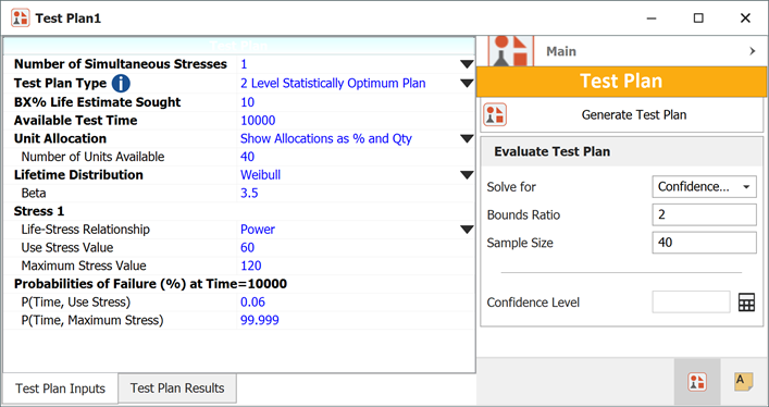
A reliability engineer is planning an accelerated test for a mechanical component. Torque is the only factor in the test. The purpose of the experiment is to estimate the B10 life (time equivalent to unreliability = 0.1) of the diodes. The reliability engineer wants to use a 2 Level Statistically Optimum Plan because it would require fewer test chambers than a 3 level test plan. 40 units are available for the test. The mechanical component is assumed to follow a Weibull distribution with beta = 3.5, and a power model is assumed for the life-stress relationship. The test is planned to last for 10,000 cycles. The engineer has estimated that there is a 0.06% probability that a unit will fail by 10,000 cycles at the use stress level of 60 N • m. The highest level allowed in the test is 120 N • m and a unit is estimated to fail with a probability of 99.999% at 120 N • m. The following setup shows the test plan in Weibull++.

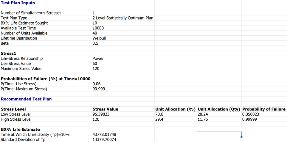
The Two Level Statistically Optimum Plan is shown next.

The Two Level Statistically Optimum Plan is to test 28.24 units at 95.39 N • m and 11.76 units at 120 N • m. The variance of the test at B10 is .

Test Plan Evaluation

In addition to assessing , the test plan can also be evaluated based on three different criteria: confidence level, bounds ratio or sample size. These criteria can be assessed before conducting the recommended test to decide whether the test plan is satisfactory or whether some modifications would be beneficial. We can solve for any one of three criteria, given the two other criteria.

The bounds ratio is defined as follows:

This ratio is analogous to the ratio that can be calculated if a test is conducted and life data are obtained and used to calculate the ratio of the confidence bounds based on the results.

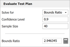
For this example, assume that a 90% confidence is desired and 40 units are to be used in the test. The bounds ratio is calculated as 2.946345, as shown next.

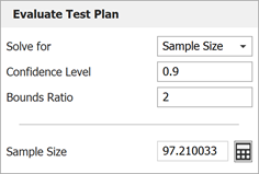
If this calculated bounds ratio is unsatisfactory, we can calculate the required number of units that would meet a certain bounds ratio criterion. For example, if a bounds ratio of 2 is desired, the required sample size is calculated as 97.210033, as shown next.

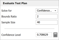
If the sample size is kept at 40 units and a bounds ratio of 2 is desired, the equivalent confidence level we have in the test drops to 70.8629%, as shown next.

Test Plans for Two Stress Types

This section presents a discussion of some of the most popular test plans used when two stress factors are applied in the test and interactions are assumed not to exists between the factors. The location parameter can be expressed as function of stresses and or as a function of their normalized stress levels as follows:

In order to design a test, the following information needs to be determined beforehand:

1. The stress limits (the design stress, and the highest test stress, ) of each stress type.

2. The test time (or censoring time), . .

3. The probability of failure at at three stress combinations. Usually , and are used ( indicates probability and the subscript represents the design stress, while represents the highest stress level in the test).

For two-stress test planning, two methods are available: the Three Level Optimum Plan and the Five Level Best Compromise Plan.

Three Level Optimum Plan

The Three Level Optimum Plan is obtained by first finding a one-stress degenerate Two Level Statistically Optimum Plan and splitting this degenerate plan into an appropriate two-stress plan. In a degenerate test plan, the test is conducted at any two (or more) stress level combinations on a line with slope that passes through the design . Therefore, in the case of a degenerate design, we have:

Degenerate plans help reducing the two-stress problem into a one-stress problem. Although these degenerate plans do not allow the estimation of all the model parameters and would be an unlikely choice in practice, they are used as a starting point for developing more reasonable optimum and compromise test plans. After finding the one stress degenerate Two Level Statistically Optimum Plan using the methodology explained in 13.4.3.1, the plan is split into an appropriate Three Level Optimum Plan.

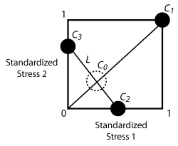
The next figure illustrates the concept of the Three Level Optimum Plan for a two-stress test. is the (0,0) point. and are the one-stress degenerate Two Level Statistically Optimum Plan. , which corresponds to ( ), is always used for this type of test and is the high stress level of the degenerate plan. corresponds to the low stress level of the degenerate plan. A line, , is drawn passing through such that all the points along the line have the same probability of failures at the end of the test with the stress levels of the plan. and are then determined by obtaining the intersections of with the boundaries of the square.

, and represent the the Three Level Optimum Plan. Readers are encouraged to review Escobar and Meeker [37] for more details about this test plan.

Five Level Best Compromise Plan

The Five Level Best Compromise Plan is obtained by first finding a degenerate one-stress Three Level Best Compromise Plan, using the methodology explained in the Three Level Best Compromise Plan (with ) , and splitting this degenerate plan into an appropriate two-stress plan.

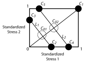
In the next figure, is the (0,0) point. and are the degenerate one-stress Three Level Best Compromise Plan. Points along the line have the same probability of failure at the end of the test plan, while points on have the same probability of failure at the end of the test plan. , and are then determined by obtaining the intersections of and with the boundaries of the square.

, , and represent the the Five Level Best Compromise Plan. Readers are encouraged to review Escobar and Meeker [37] for more details about this test plan.