Warranty Data Analysis Example
This example validates the results of a warranty data analysis in a Weibull++ warranty folio.
Reference Case
The data set is from Example 11.2 on page 453 in the book Life Cycle Reliability Engineering by Dr. Guangbin Yang, John Wiley & Sons, 2007.
Data
A Nevada chart for the warranty data is provided in Table 11.3. The last two rows were combined, as specified in the example.
| TTF | ||||||||||||||
|---|---|---|---|---|---|---|---|---|---|---|---|---|---|---|
| TIS | 1 | 2 | 3 | 4 | 5 | 6 | 7 | 8 | 9 | 10 | 11 | 12 | Total | Sales Volume |
| 12 | 3 | 0 | 3 | 3 | 4 | 2 | 1 | 5 | 4 | 2 | 3 | 3 | 45 | 2123 |
| 11 | 0 | 1 | 2 | 0 | 4 | 2 | 1 | 2 | 0 | 4 | 3 | 30 | 1853 | |
| 10 | 1 | 3 | 2 | 2 | 3 | 4 | 3 | 5 | 4 | 8 | 45 | 2238 | ||
| 9 | 1 | 2 | 0 | 3 | 4 | 2 | 2 | 3 | 6 | 32 | 3052 | |||
| 8 | 2 | 3 | 2 | 6 | 2 | 1 | 6 | 4 | 34 | 2953 | ||||
| 7 | 1 | 1 | 3 | 2 | 1 | 4 | 8 | 27 | 2788 | |||||
| 6 | 1 | 0 | 1 | 0 | 1 | 2 | 11 | 2037 | ||||||
| 5 | 0 | 0 | 1 | 1 | 0 | 7 | 1863 | |||||||
| 4 | 0 | 0 | 1 | 1 | 6 | 1231 | ||||||||
| 3 | 0 | 1 | 1 | 5 | 823 | |||||||||
| 2 | 0 | 1 | 3 | 638 | ||||||||||
| 1 | 0 | 1 | 568 | |||||||||||
| Total | 9 | 12 | 16 | 18 | 19 | 17 | 21 | 19 | 14 | 14 | 6 | 3 | ||
Result
The book first converted the data in the table above into the following format, as given in Table 11.4 in the book.
| TTF (Months) | Number of Failures | Number of Censored Units |
|---|---|---|
| 1 | 9 | 568 |
| 2 | 12 | 637 |
| 3 | 16 | 821 |
| 4 | 18 | 1229 |
| 5 | 19 | 1861 |
| 6 | 17 | 2032 |
| 7 | 21 | 2768 |
| 8 | 19 | 2927 |
| 9 | 14 | 3029 |
| 10 | 14 | 2203 |
| 11 | 6 | 1834 |
| 12 | 3 | 2090 |
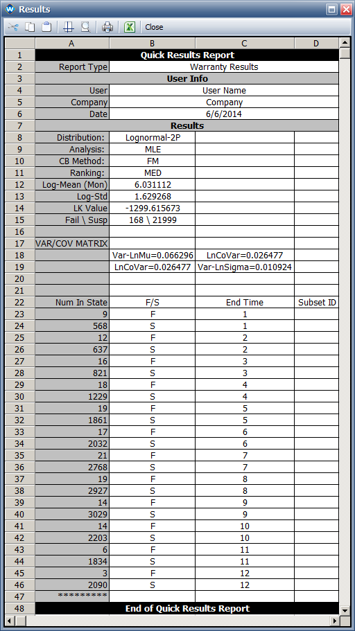
A lognormal distribution is used and the fitted model parameters are: Ln-Mean = 6.03 and Ln-Std = 1.63.
Results in Weibull++
In Weibull++, the data set is entered into a warranty folio, using the Nevada chart format. The following pictures show the sales and returns data.
The following picture shows the parameters of the lognormal distribution and its associated failure/suspension data. The results are the same as the results shown in the book.
The following picture shows the probability plot of the lognormal distribution.


