Degradation Data Analysis with a Linear Regression Model
This example validates the results for a degradation analysis with a linear regression model in Weibull++ degradation folios.
Reference Case
The data set is from Example 13.10 on page 338 in the book Statistical Methods for Reliability Data by Dr. Meeker and Dr. Escobar, John Wiley & Sons, 1998.
Data
The test is for the current (i.e., amperage) of a laser device. Failure is defined as a 10% increases in amperage.
| Time | Unit Number | ||||||||||||||
|---|---|---|---|---|---|---|---|---|---|---|---|---|---|---|---|
| 1 | 2 | 3 | 4 | 5 | 6 | 7 | 8 | 9 | 10 | 11 | 12 | 13 | 14 | 15 | |
| 250 | 0.47 | 0.71 | 0.71 | 0.36 | 0.27 | 0.36 | 0.36 | 0.46 | 0.51 | 0.41 | 0.44 | 0.4 | 0.3 | 0.44 | 0.51 |
| 500 | 0.93 | 1.22 | 1.17 | 0.62 | 0.61 | 1.39 | 0.92 | 1.07 | 0.93 | 1.79 | 1 | 0.8 | 0.74 | 0.7 | 0.83 |
| 750 | 2.11 | 1.9 | 1.73 | 1.36 | 1.11 | 1.95 | 1.21 | 1.42 | 1.57 | 2.38 | 1.57 | 1.4 | 1.52 | 1.05 | 1.29 |
| 1000 | 2.72 | 2.3 | 1.99 | 1.95 | 1.77 | 2.86 | 1.46 | 1.77 | 1.96 | 3 | 1.96 | 1.7 | 1.85 | 1.35 | 1.52 |
| 1250 | 3.51 | 2.87 | 2.53 | 2.3 | 2.06 | 3.46 | 1.93 | 2.11 | 2.59 | 3.84 | 2.51 | 3 | 2.39 | 1.8 | 1.91 |
| 1500 | 4.34 | 3.75 | 2.97 | 2.95 | 2.58 | 3.81 | 2.39 | 2.4 | 3.29 | 4.5 | 2.84 | 3.6 | 2.95 | 2.55 | 2.27 |
| 1750 | 4.91 | 4.42 | 3.3 | 3.39 | 2.99 | 4.53 | 2.68 | 2.78 | 3.61 | 5.25 | 3.47 | 4 | 3.51 | 2.83 | 2.78 |
| 2000 | 5.48 | 4.99 | 3.94 | 3.79 | 3.38 | 5.35 | 2.94 | 3.02 | 4.11 | 6.26 | 4.01 | 4.4 | 3.92 | 3.39 | 3.42 |
| 2250 | 5.99 | 5.51 | 4.16 | 4.11 | 4.05 | 5.92 | 3.42 | 3.29 | 4.6 | 7.05 | 4.51 | 4.8 | 5.03 | 3.72 | 3.78 |
| 2500 | 6.72 | 6.07 | 4.45 | 4.5 | 4.63 | 6.17 | 4.09 | 3.75 | 4.91 | 7.8 | 4.8 | 5.2 | 5.47 | 4.09 | 4.11 |
| 2750 | 7.13 | 6.64 | 4.89 | 4.72 | 5.24 | 7.7 | 4.58 | 4.16 | 5.34 | 8.32 | 5.2 | 5.5 | 5.84 | 4.83 | 4.38 |
| 3000 | 8 | 7.16 | 5.27 | 4.98 | 5.62 | 8.61 | 4.84 | 4.76 | 5.84 | 8.93 | 5.66 | 6 | 6.5 | 5.41 | 4.63 |
| 3250 | 8.92 | 7.78 | 5.69 | 5.28 | 6.04 | 9.15 | 5.11 | 5.16 | 6.4 | 9.55 | 6.2 | 6.2 | 6.94 | 5.76 | 5.38 |
| 3500 | 9.49 | 8.42 | 6.02 | 5.61 | 6.32 | 9.95 | 5.57 | 5.46 | 6.84 | 10.5 | 6.54 | 7 | 7.39 | 6.14 | 5.84 |
| 3750 | 9.87 | 8.91 | 6.45 | 5.95 | 7.1 | 10.49 | 6.11 | 5.81 | 7.2 | 11.3 | 6.96 | 7.4 | 7.85 | 6.51 | 6.16 |
| 4000 | 10.94 | 9.28 | 6.88 | 6.14 | 7.59 | 11.01 | 7.17 | 6.24 | 7.88 | 12.2 | 7.42 | 7.9 | 8.09 | 6.88 | 6.62 |
Result
The book provides a linear regression model,
, but the parameters of the model are not provided. Only the predicted failure times are given. These are: 3702, 4194, 5847, 6172, 5301, 3592, 6051, 6538, 5110, 3306, 5326, 4995, 4721, 5689, and 6102. A Weibull distribution is used to fit the data; however, the model parameters are not provided. Only a probability plot is given.
Results in Weibull++
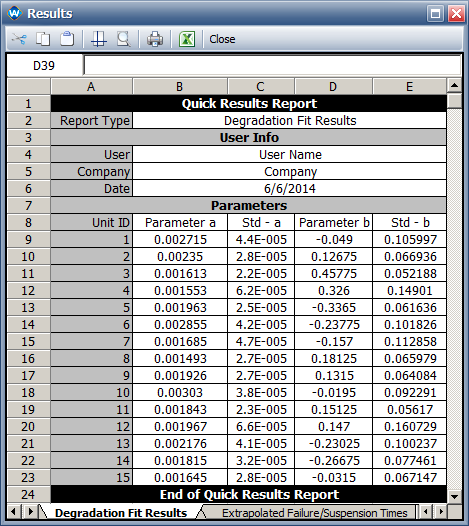
- The following picture shows the parameters of the linear regression model for each unit.
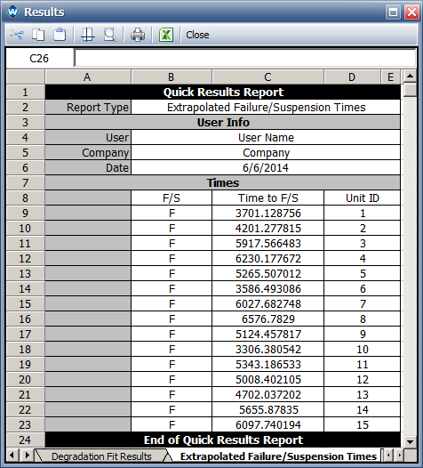
- The predicted pseudo failure times are shown next.
- The predicted failure times in Weibull++ are slightly different from the values given in the book. Since the book does not provide the model parameters, we couldn’t compare the Weibulll++ results with the results in the book.
- The next picture shows the parameters of the fitted Weibull distribution.


