Reliability Allocation and Optimization using BlockSim
In last month's Reliability Basics article, we discussed some popular reliability allocation methods, including the equal, AGREE, ARINC, feasibility of objectives and repairable systems apportionment techniques. We also presented some practical applications using ReliaSoft's Lambda Predict software. All of the methods discussed are based on the assumptions that:
- The components' lifetime characteristics are described by the exponential distribution; in other words, the components all exhibit a constant failure rate behavior.
- The components are all connected in a series configuration reliability-wise.
These methodologies are widely used in many reliability prediction standards and are useful when limited reliability data exists, usually during the initial design phase of a new product. When there are specific details concerning the failure rate behavior of the product and there is a more complex configuration instead of just components in series, we can go one step further and incorporate a more detailed analysis of reliability allocation that is free of the above assumptions. In this article we present a more advanced method for reliability allocation that is free of these assumptions and can be performed with ReliaSoft's BlockSim 7 software.
In BlockSim, we can create complex reliability block diagrams that model advanced systems. A reliability block diagram represents the reliability relationships of the components in a system and can comprise blocks in any combination of series, parallel, stand-by and load sharing configurations. After constructing the reliability model of a complex system, we can optimize the allocation of reliability to different components in order to meet a reliability specification while considering the cost of the allocation.
Reliability Improvement Methodology in BlockSim
There are two approaches when trying to improve the reliability of a system: fault avoidance and fault tolerance. Fault avoidance is achieved by using highly reliable components, and fault tolerance is achieved by adding redundancy. Note that although adding redundancy can sometimes be the easiest way to achieve a goal, it is not always the preferred solution, since it can result in greater system complexity and additional product costs due to the increased weight or size.
The optimum method of allocating reliability should take into account the cost or relative difficulty of improving the reliability of different subsystems or components. That way we are not simply allocating reliability to components, but are solving the optimization problem of the most cost-effective and efficient way of allocating or improving reliability in order to meet the required system goal. Note that reliability requirements are always associated with a specific mission duration, since reliability is defined as a function of a specified lifetime variable, such as time, cycles, miles etc.
BlockSim uses the following default cost function that acts like a penalty function for increasing a component's reliability. It is assumed that the cost increases exponentially since it is more difficult to progressively increase reliability:

where:
- Ci(Ri) is the penalty (or cost) equation as a function of component reliability.
- f is the feasibility (or cost index) of improving a component's reliability relative to the other components in the system.
- Rmin,i is the current reliability at the time at which the optimization is to be performed.
- Rmax,i is the maximum achievable reliability at the time at which the optimization is to be performed.
The feasibility term is a constant that represents the difficulty in increasing a component's reliability relative to the rest of the components in the system. Depending on the design complexity, technological limitations, etc., certain components can be very hard to improve. Clearly, the more difficult it is to improve the reliability of the component, the greater the cost. The lower the feasibility value, the more rapidly the cost function approaches infinity.
The expression for the overall system cost at the system reliability goal is the sum of the costs of its components:

Once the overall cost function for the system has been defined, the problem becomes one of minimizing the cost function while remaining within the constraints defined by the target system reliability and the reliability ranges for the components.
BlockSim employs a nonlinear programming technique to minimize the system cost function. The structural properties of the system are accounted for in the determination of the optimum solution. For example, the optimization for a system of three units in series will be different from the optimization for a system consisting of the same three units in parallel, in spite of the fact that the cost functions for the individual components remain the same. The optimization occurs by varying the reliability values of the components within their respective constraints of maximum and minimum reliability in such a way that the overall system goal is achieved at the minimum overall system cost.
Example
Let's examine the allocation and optimization method in BlockSim 7 through an example. Suppose that we have the reliability block diagram that is shown in Figure 1.
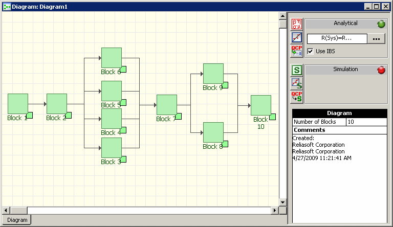
Figure 1: A Reliability Block Diagram in BlockSim
This block diagram is composed of 10 blocks that are in a mix of series and parallel configurations. None of the blocks has a constant failure rate. Based on these two facts, the reliability allocation methods described in last month's HotWire article cannot be applied to this system.
The lifetime characteristics of each block are entered by double-clicking the block. For example, Figure 2 shows that Block 1 follows a Weibull distribution with a shape parameter beta equal to 2.5 and a characteristic life eta equal to 2000.
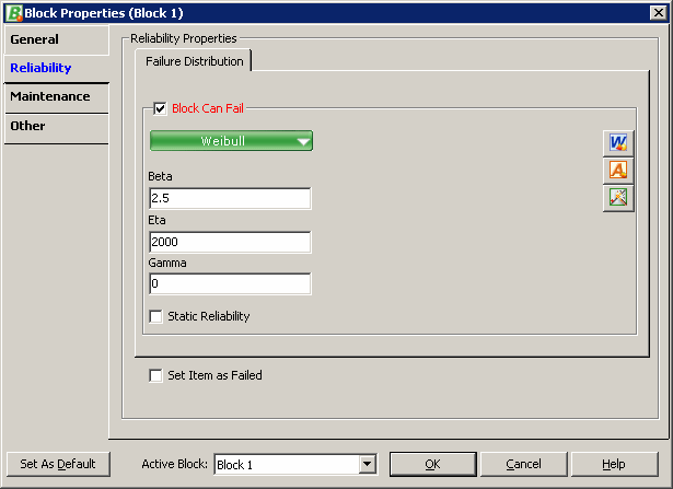
Figure 2: Failure Distribution for Block 1
BlockSim can also link to Weibull++ or ALTA Folios so that test results for specific components can be applied directly to the block. For example, by clicking the Weibull++ icon on the Reliability tab of the Block Properties window for Block 6, we can apply lifetime characteristics based on the distribution and its associated parameters previously identified from component level life data analysis.

(Clicking the ALTA icon would allow us, instead, to apply calculated results from accelerated testing.). Figure 3 shows the component level testing results for Block 6.
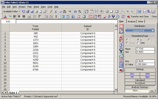
Figure 3: Estimating Lognormal Distribution Parameters for
Block 6 by Associating a Weibull++ Folio
We associate this life data analysis Folio with Block 6 by clicking the Transfer and Close button. The parameters of the associated lognormal distribution are automatically applied to the failure distribution properties for the specific block, as shown in Figure 4.
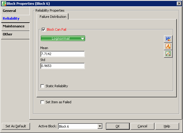
Figure 4: Applying the Associated Life Data Analysis Results
for Block 6
The failure distributions for all of the blocks are as follows:
Block 1: Weibull β=2.5;
η=2000,
γ=0
Block 2: Weibull β=3;
η=2500,
γ=0
Block 3: Weibull β=1.5;
η=3000,
γ=0
Block 4: Weibull β=1.9;
η=5000,
γ=0
Block 5: Exponential μ=5000,
γ=0
Block 6: Lognormal μ=7.7142,
σ=0.9653
Block 7: Lognormal μ=7,
σ=1
Block 8: Weibull β=0.9;
η=5000,
γ=0
Block 9: Weibull β=5;
η=6120,
γ=0
Block 10: Weibull β=4.5;
η=7000,
γ=0
We can define these for each block using the methods shown above.
BlockSim can calculate very complex reliability equations based on the different configurations. The equation below is the system reliability equation for the specific configuration shown in Figure 1:

So far, we have defined a complex system configuration and defined the different failure distributions for each of the 10 blocks. Suppose that we have a system reliability specification of Rsystem = 90% at mission end time = 1000. Using the Quick Calculation Pad, we find that the system reliability at t = 1000 is 42.17%, as shown in Figure 5.

Figure 5: Calculating System Reliability at t = 1000
The question now is which components to redesign for increased reliability (fault avoidance) or which components to duplicate in parallel configurations (fault tolerance) in order to meet the specific reliability requirement at t = 1000.
To determine this, for each block to be used in the optimization process (in this case, all blocks), we select the Block to be used in optimized allocation option on the Reliability Allocation page of the Other tab in the Block Properties window. We then define a maximum achievable reliability for each component, which, as described in the methodology section, is a limiting reliability that the component will approach but not reach, usually dictated by technological or financial constraints. It is important to note that the time associated with this maximum achievable reliability is the same as that of the overall system reliability goal, in this case a mission duration t = 1000. We also choose a feasibility factor for each of the blocks. For example, for Block 4, the maximum achievable reliability is 0.999 and the slider is moved to 7 on a scale of 1 to 9, meaning that it is between moderate and hard to improve reliability for Block 4, as compared to the rest of the blocks.
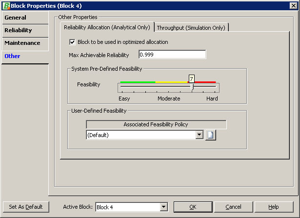
Figure 6: Reliability Allocation Properties for Block 4
Note that the feasibility used in the cost function for a particular block is given by f = 1 slider value/100, so the feasibility associated with Block 4 is 0.3.
Once these properties have been specified for all 10 blocks, we can use the optimization page of the Quick Calculation Pad. As shown in Figure 7, we define the mission end time of interest, 1000, and the associated reliability goal of 90%.
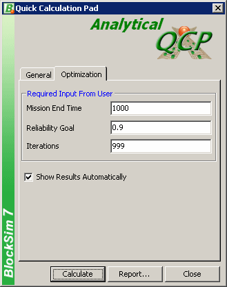
Figure 7: Optimization in the QCP
Figure 8 shows the results of the optimization process.
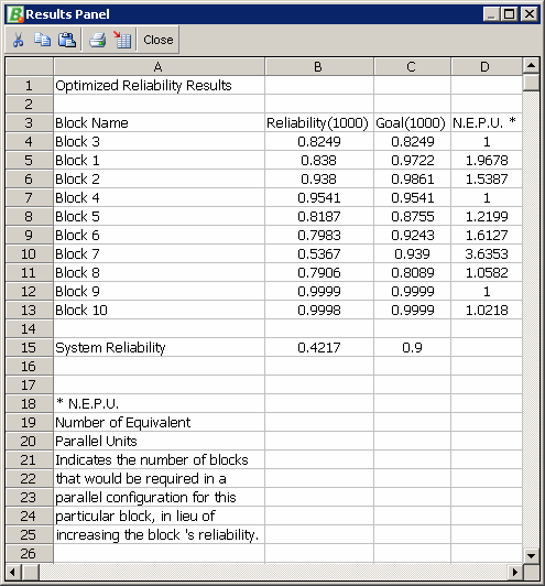
Figure 8: Reliability Optimization Results for t = 1000
Column C shows the calculated goal for each of the blocks in terms of fault avoidance. In other words, the values in Column C represent the new optimized goal for each of the blocks so that the 90% system reliability requirement at t = 1000 is met. Column D presents the optimization results in terms of fault tolerance. In other words, the values in Column D represent the number of equivalent parallel units that would have to be used to meet the 90% system reliability goal if the reliability of those units could not be increased from the values in Column B. The system configuration, the specific failure distributions for each block, the feasibility factors and the maximum achievable reliability values have all been factored in to provide the optimum reliability improvement combination to meet the predefined goal.
Conclusion
In this article we presented a powerful way of allocating and optimizing reliability using the methodology in ReliaSoft's BlockSim 7. This approach can handle any type of system configuration and it does not require unrealistic assumptions concerning constant failure rates. It uses a non-linear optimization method to identify the most cost-effective and efficient way to achieve a system reliability goal.
References
[1] ReliaSoft Corporation, System Analysis Reference,
Tucson, AZ: ReliaSoft Publishing, 2007, pp. 174-197.
[2] ReliaSoft Corporation, "Reliability
Allocation and Optimization," Reliability HotWire,
Issue 6, August 2001.
[3] ReliaSoft Corporation, "Reliability
Allocation Using Lambda Predict," Reliability HotWire,
Issue 98, April 2009.
[4] Mettas, A., "Reliability Allocation and Optimization for
Complex Systems," Proceedings of the Annual Reliability &
Maintainability Symposium, 2000.